• Advanced Photonics
  • Vol. 3, Issue 3, 035001 (2021)
Jia Tan1、†, Shengliang Xu1, Xu Han1, Yueming Zhou1、*, Min Li1, Wei Cao1, Qingbin Zhang1、*, and Peixiang Lu1、2、*
Author Affiliations
  • 1Huazhong University of Science and Technology, School of Physics and Wuhan National Laboratory for Optoelectronics, Wuhan, China
  • 2Wuhan Institute of Technology, Hubei Key Laboratory of Optical Information and Pattern Recognition, Wuhan, China
  • show less
    DOI: 10.1117/1.AP.3.3.035001 Cite this Article Set citation alerts
    Jia Tan, Shengliang Xu, Xu Han, Yueming Zhou, Min Li, Wei Cao, Qingbin Zhang, Peixiang Lu. Resolving and weighing the quantum orbits in strong-field tunneling ionization[J]. Advanced Photonics, 2021, 3(3): 035001 Copy Citation Text show less
    (a)–(c) The experimentally measured PEMDs for strong-field tunneling ionization of Ar by the parallel two-color (800 nm+400 nm) field with relative phase φ=0, 0.5π, and 1.5π, respectively. The laser intensities of the FM and SH fields are 1.2×10¹⁴ and 0.3×10¹¹ W/cm2, respectively. (d)–(f) NDs for the distributions in (a)–(c) (see text for details).
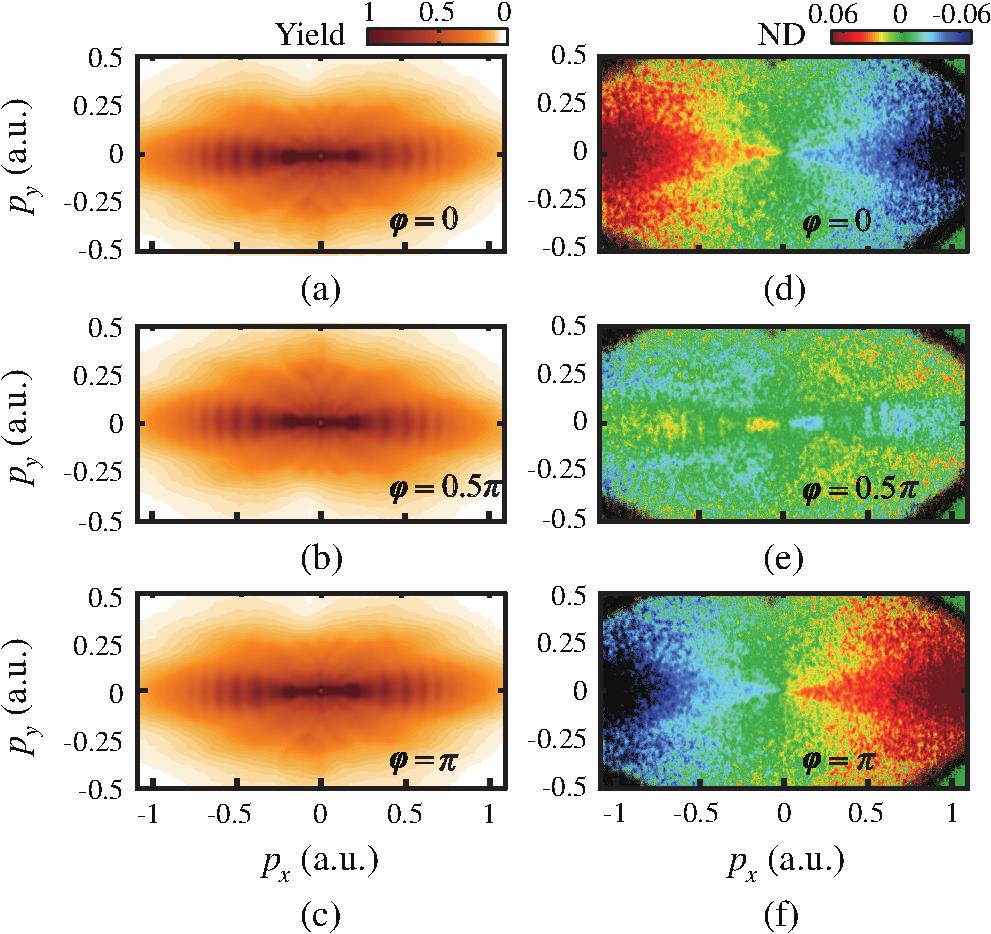
    Fig. 1. (a)–(c) The experimentally measured PEMDs for strong-field tunneling ionization of Ar by the parallel two-color (800  nm+400  nm) field with relative phase φ=0, 0.5π, and 1.5π, respectively. The laser intensities of the FM and SH fields are 1.2×10¹⁴ and 0.3×10¹¹  W/cm2, respectively. (d)–(f) NDs for the distributions in (a)–(c) (see text for details).
    (a) The ND as a function of φ for the momentum (px,py)=(−0.6,0.1) a.u. The open circles show the experimental data and the green curve shows the fitted results. (b) The fitted ND by Eq. (2) as a function of φ for the momentum (px,py)=(−0.6,0) (blue curve), (−0.6,0.1) (purple curve), and (−0.6,0.2) a.u. (green curve). The data are normalized such that the maximum of each curve is unity. (c) Same as (b) but for (px,py)=(−0.4,0) (black curve), (−0.5,0) (red curve), and (−0.6,0) a.u. (yellow curve). (d) The optimal phase φm in the region of px∈[−1.1,1.1] a.u. and py∈[−0.5,0.5] a.u. (e) Cuts of φm at px=−0.4 a.u. (red crosses), −0.5 a.u. (green squares), and −0.6 a.u. (blue triangles). The error bars show the 95% confidence interval in fitting.
    Fig. 2. (a) The ND as a function of φ for the momentum (px,py)=(0.6,0.1) a.u. The open circles show the experimental data and the green curve shows the fitted results. (b) The fitted ND by Eq. (2) as a function of φ for the momentum (px,py)=(0.6,0) (blue curve), (0.6,0.1) (purple curve), and (0.6,0.2) a.u. (green curve). The data are normalized such that the maximum of each curve is unity. (c) Same as (b) but for (px,py)=(0.4,0) (black curve), (0.5,0) (red curve), and (0.6,0) a.u. (yellow curve). (d) The optimal phase φm in the region of px[1.1,1.1] a.u. and py[0.5,0.5] a.u. (e) Cuts of φm at px=0.4 a.u. (red crosses), 0.5 a.u. (green squares), and 0.6 a.u. (blue triangles). The error bars show the 95% confidence interval in fitting.
    (a) Illustration of the ionization times of the long and short orbits in strong-field tunneling ionization. The long and short orbits correspond to the ionization events, where the electron is released at the falling and rising edges of electric field, respectively. The blue curve indicates the electric field of the FM field and the red curve shows its vector potential. (b) The ND(p;φ) for the long orbit with transverse momentum py=0, calculated by CCSFA. The solid red curve indicates the optimal phase φmL. (c) The same as (b) but for the short orbit. The black arrow denotes the phase window formed by φmL and φmS. (d) The optimal phase φmL of the long orbit for px∈[−1,−0.2] a.u. and py∈[−0.36,0.36] a.u. (e) The same as (d) but for the short orbit.
    Fig. 3. (a) Illustration of the ionization times of the long and short orbits in strong-field tunneling ionization. The long and short orbits correspond to the ionization events, where the electron is released at the falling and rising edges of electric field, respectively. The blue curve indicates the electric field of the FM field and the red curve shows its vector potential. (b) The ND(p;φ) for the long orbit with transverse momentum py=0, calculated by CCSFA. The solid red curve indicates the optimal phase φmL. (c) The same as (b) but for the short orbit. The black arrow denotes the phase window formed by φmL and φmS. (d) The optimal phase φmL of the long orbit for px[1,0.2] a.u. and py[0.36,0.36] a.u. (e) The same as (d) but for the short orbit.
    (a) The ND at (px,py)=(−0.5,0) a.u. as a function of φ. The solid green and purple curves show the theoretical results of the signal from the long and short orbits, respectively. The black squares represent the experimental data, where both the long and short orbits contribute. The dashed blue lines indicate the optimal phases φmL and φmS, and the blue arrow denotes their phase window. (b) The same as (a) but for (px,py)=(−0.5,0.2) a.u. (c) The ratios α/β extracted from the experimental data. (d) The cuts of α/β at px=−0.4 (red circles), −0.6 (green squares), and −0.95 a.u. (purple triangles), respectively.
    Fig. 4. (a) The ND at (px,py)=(0.5,0) a.u. as a function of φ. The solid green and purple curves show the theoretical results of the signal from the long and short orbits, respectively. The black squares represent the experimental data, where both the long and short orbits contribute. The dashed blue lines indicate the optimal phases φmL and φmS, and the blue arrow denotes their phase window. (b) The same as (a) but for (px,py)=(0.5,0.2) a.u. (c) The ratios α/β extracted from the experimental data. (d) The cuts of α/β at px=0.4 (red circles), 0.6 (green squares), and 0.95 a.u. (purple triangles), respectively.
    Jia Tan, Shengliang Xu, Xu Han, Yueming Zhou, Min Li, Wei Cao, Qingbin Zhang, Peixiang Lu. Resolving and weighing the quantum orbits in strong-field tunneling ionization[J]. Advanced Photonics, 2021, 3(3): 035001
    Download Citation