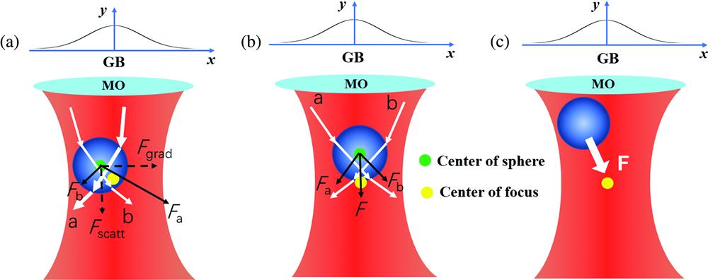
Fig. 1. Schematic diagram of optical tweezers: (a) when the particle is away from the center of the beam focus, (b) when the particle is slightly above the center of the beam focus, and (c) net force acting on the dielectric sphere. Fa and Fb are the forces produced by the refracted rays a and b, respectively. Fgrad and Fscat denote the gradient force and scattering force, respectively. GB, Gaussian beam; MO, microscope objective.

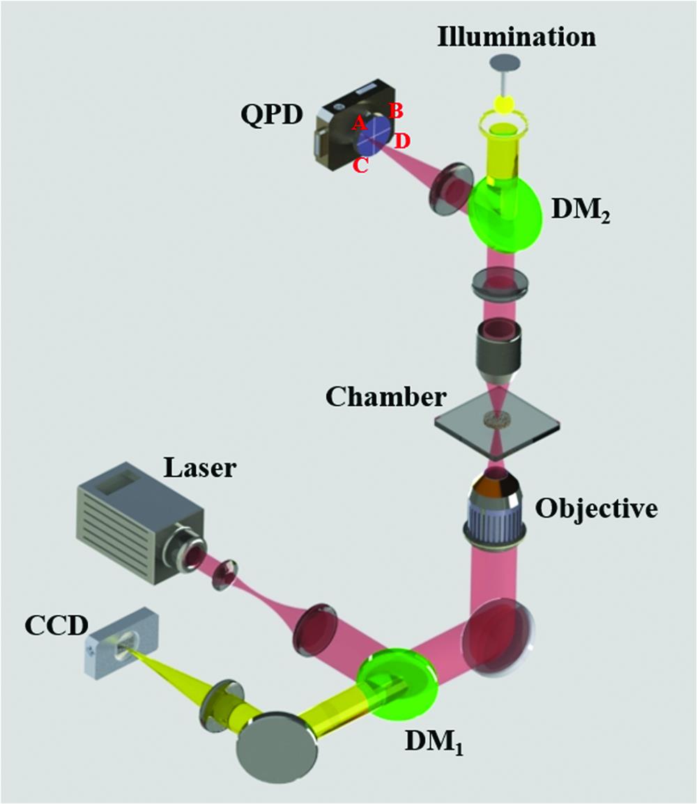
Fig. 2. Experimental configuration of conventional optical tweezers. A simple telescope is used to expand the laser beam to overfill the back aperture of the objective. The expanded laser beam, reflected by a dichroic mirror (DM1), is coupled into the objective. The laser beam is focused by the objective and forms an optical trap. The QPD is placed in a conjugate plane of the condenser, to collect the forward scattered light that is reflected by the dichroic mirror (DM2). The trapped particles are imaged with a CCD camera. The lateral (x,y) position of the particle can be measured by the normalized output voltage signals from the four quadrants, namely, x=(A+D)−(B+C)A+B+C+D and y=(A+B)−(C+D)A+B+C+D.

Fig. 3. Optical trapping of birefringent microparticles that show the transfer of OAM and SAM. (a) The trapped particle is spinning counterclockwise about its own axis (left column) and orbiting clockwise about the beam’s axis (right column) separately. Adapted from Ref. 58. (b) The particle rotates around its own axis (left column) and the beam’s axis (right column) simultaneously. Adapted from Ref. 59.

Fig. 4. Transverse intensity profiles of LG modes with (a) LG00, (b) LG01, (c) LG20, and (d) LG22. The color denotes the normalized intensity distribution.

Fig. 5. Transverse intensity profiles of Bessel beams and its Fourier transform with (a) ℓ=0 and (b) ℓ=1. The color denotes the normalized intensity distribution.

Fig. 6. Transverse intensity distribution of perfect vortex beams with topological charge ℓ=1, 4, 10, and 15. Here, ρ0 is the radius of the ring-like intensity profile and Δρ its width. Notice that the intensity profile remains constant as ℓ increases. The color represents the normalized intensity distribution.

Fig. 7. Transverse intensity pattern of a truncated zeroth-order Mathieu beam with (a) even and (b) odd modes. The color represents the normalized intensity distribution.

Fig. 8. Airy beam profiles. (a) Parabolic trajectory and (b) transverse intensity profile of an Airy beam with infinite energy compared with those of a finite energy Airy beam in (c) and (d). The color represents the normalized intensity distribution.

Fig. 9. Transverse intensity distribution of low-order (a) even and (b) odd IG modes with ϵ=2, z=0, and ω0=1mm. The color represents the normalized intensity distribution.

Fig. 10. Intensity distribution of an HC beam from numerical simulations. (a), (c) The near-field intensity distribution; (b), (d) the far-field. (a), (b) K=0; (c), (d) K=1. In all cases, ℓ=50. The color represents the normalized intensity distribution.

Fig. 11. Intensity and polarization distribution of the fundamental cylindrical vector beams. (a) Radial, (b) hybrid odd, (c) azimuthal, and (d) hybrid even modes. The color represents the normalized intensity distribution, while the lines are associated with the polarization orientation of the electric field.

Fig. 12. Optical trapping and control of 3D structures using superpositions of LG0ℓ and LG0−ℓ as the trapping beam. (a) Two microspheres trapped at the two bright spots created by the superposition of the modes LG01 and LG0−1. (b) Trapping and release of eight microspheres trapped along the beam’s propagation axis by the intensity pattern generated by superposed modes of LG02 and LG0−2, as schematically shown in (d). (c) Rotation of the eight-microsphere cubic structure. (e) Schematic representation of the generation of 3D structures containing a larger number of microspheres. Adapted from Ref. 110.

Fig. 13. Optical trapping and rotations in counterpropagating circularly polarized LG beams of silicon nanowires aligned (a) parallel and (b) perpendicular to the beam propagation axis, where orbiting and orbiting-reorientation are shown, respectively. The simultaneous spinning and orbiting of a shorter nanowire is shown in (c) and (d). Adapted from Ref. 111.

Fig. 14. Anomalous motion of a particle trapped in strongly focused high-order LG beams. (a) The intensity profile of the LG beam with topological charge 3. (b) The plot of the distribution of the radiation force exerted on the trapped particle for different center-of-mass radii. (c) The radial (blue line) and azimuthal (red broken line) components of the radiation force for different radii of the trapped particles. Adapted from Ref. 113.

Fig. 15. Rotation of a polystyrene bead and a glass sliver trapped with an LG mode of ℓ=±30. (a) Sequential images of these particles showing their direction of rotation. (b) Angular velocity of each particle with respect to the topological charge. Adapted from Ref. 114.

Fig. 16. Optical trapping with Bessel beams. (a) Trapping of multiple particles at different optical planes. Adapted from Ref. 68. (b) Trapping and delivering of two particles using a sliding Bessel standing beam. Adapted from Ref. 118.

Fig. 17. (a) Schematic representation of optical trapping with frozen waves in multiple parallel planes. Sequence of (a1)–(d1) one and (a2)–(d2) two microparticles (orange circle) trapped at different transverse planes along the propagation direction. Adapted from Ref. 120.

Fig. 18. Effect of the size of the trapped particle on optical trapping with vortex beams. (a)–(c) Optical forces of a particle with different sizes compared to the radius of the bright rings of Bessel vortex beams. The blue circle and blue dot denote the edge and the center of the trapped particle. The cyan contour denotes the zero force azimuthal directions. The magenta lines represent the deterministic trajectory of a particle. (d) Illustration of a rotation of a single silver nanowire trapped by an LG vortex beam. (a)–(c) Adapted from Ref. 121. (d) Adapted from Ref. 122.

Fig. 19. (a) A perfect vortex beam with ℓ=25 and (b) the beam with the scattered light from a single trapped particle. (c) Linear relationship between the particle rotation rate and the integer topological charge. (d) Snapshot of a trapped particle rotating around the circumference of a perfect vortex beam indicated by the red circle. (e) Angular velocity of the particle as a function of its angular position. Adapted from Refs. 123 and 124.

Fig. 20. Optical trapping of nonspherical particles. (a) Mathieu beam with m=4. (b) 3D intensity distribution. (c) Particles orientation within transversal intensity distribution. (d) Rotating hologram and (e) corresponding Mathieu beam. (f) Time-lapse images of trapped particles depending on the orientation of the Mathieu beam and (g) their corresponding schematics. Adapted from Ref. 125.

Fig. 21. Optical manipulation with Airy beams. (a) Schematic representation of a microparticle being transported along a parabolic trajectory. Adapted from Ref. 128. Transporting particles (b) from quadrant two (green) to quadrant three (purple) and (c) from quadrant three to quadrant two. Adapted from Ref. 129. (d) The y−z plane intensity profile of a circular Airy vortex beam. (e) Rotation of the trapped silica particles on the primary ring of circular Airy vortex beam for topological charge 12. The white and yellow circles denote the vortex ring position and the position of a selected trapped particle at different time. Adapted from Ref. 130.

Fig. 22. Micromanipulation with IG beams. The top row shows the transverse intensity patterns of the beams, while the bottom row shows trapped microparticles with the corresponding beams. (a) IG5,5o mode. (b) IG2,2o mode with four columns of particles stacked along its beam axis. (c) IG4,2o mode where the four central petals close to each other show no stable traps. (d) IG14,14e mode with particles trapped at certain locations. Adapted from Ref. 132.

Fig. 23. Optical manipulation with HC beams. (a) Schematic representation of the setup required for beam generation. (b) Time-lapse images of a microbead trapped and guided along with the maximum intensity of the beam, as illustrated on the left. Adapted from Ref. 133.

Fig. 24. Optical tweezer arrays using computer-generated holograms. (a) Schematic representation of the fields at the input hologram and output Fourier planes, where k is the wave vector. (b) DOE (the black color represents a phase shift of π-rad) etched on a fused silica substrate for a hexagonal array of traps. (c) 19 silica spheres (1-μm diameter) trapped in the hexagonal array. Adapted from Ref. 135. (d) Typical experimental setup for optical tweezers using computer-generated holograms. A telescope relays the plane of the diffraction grating to the input pupil of the microscope objective. In this way, multiple beams generated by the diffraction grating can create multiple optical traps. The bottom left inset shows an example of a phase grating capable of generating an array of 20 by 20 optical traps. The bottom right inset shows the optical trapping of multiple polystyrene spheres (800 nm in diameter) in water. Adapted from Ref. 136.

Fig. 25. Optical trapping with complex optical patterns. (a) Experimentally generated beam patterns with different modes. (b) Two particles being guided along the trajectory shown by the dotted line. Adapted from Ref. 142

Fig. 26. Optical trapping with a parabolic phase gradient. Two silica beads (1.5μm in diameter) trapped in (a1) positive and (b1) negative parabolic phase gradients and (a2), (b2) the corresponding beam intensity profiles at the trapping plane. A cross-section of the beams in the x−z plane, showing (a3) the divergence and (b3) convergence of the phase gradient. Adapted from Ref. 76.

Fig. 27. Optical manipulation with 3D solenoid beams propagating parallel to the z axis. (a) Theoretical and (b) experimental profiles of the beam in 3D. (c) Experimental trajectories of trapped particles transported downward (ℓ=+30) or upward (ℓ=−30) along with the helical intensity profile in the optical solenoid beam. Adapted from Ref. 146.

Fig. 28. Optical trapping and transporting of microparticles along 3D parametrized trajectories. (a) Particles trapped along a single ring in 3D. (b) Schematic representation of (a). (c) Experimental intensity distribution of two tilted ring traps with opposite inclination. (d) Colloidal silica spheres trapped in the two rings of (c). (e) Schematic 3D representation of the knotted rings of (c) and (d). Adapted from Ref. 147.

Fig. 29. Optical trapping with arbitrary 3D parametrized curves of the beam. (a) Phase profile of a ring trap with topological charge m=30 and (b) a triangle trap with topological charge m=34. (b1) An expanded view of a section in (b), where the black arrows indicate the vector field gradient. (c) Phase gradient modulus corresponding to the beam in (b), where SP1 and SP2 indicate stationary points where the modulus is maximum and minimum, respectively. The top right images show 2D intensity profiles of the focused beam in the x−y and x−z planes. (d) Schematic representation of the optical tweezers, where the beam is focused into a sample cell containing silica beads of 1μm through a microscope objective with NA=1.4. Adapted from Ref. 149.

Fig. 30. Optical trapping with 3D toroidal-spiral beams. (a) Time-lapse images of trapped microparticles moving along the beam over 7 s, which results in (b) a decagon trajectory. (c) 3D schematic representation of the toroidal-spiral curve, where the color scheme indicates the axial z position of the curve. (d) Intensity profiles of the toroidal beam at two different axial planes. Adapted from Ref. 149.

Fig. 31. Example of a Beziér parametric curve and its application to reconfigure in real-time the trajectory of microparticles. (a) Construction of a parametric curve using (left) Beziér splines, (middle) intensity, and (left) phase of a laser beam following this parametric curve. (b) Example of real-time reconfiguration of the curve shown in (a) and its application in a real-time reconfigurable optical trap (middle). Adapted from Ref. 151.

Fig. 32. (a) Schematic representation of cylindrical vector beams under tight focusing conditions. Tightly focused vector beams with (b) radial polarization and (c) azimuthal polarization. Adapted from Ref. 159.

Fig. 33. Generation of vector beam arrays. (a) Experimental intensity profiles and (b) polarization distribution of nine vector beams generated from a single hologram. (c) Schematic representation of the experimental setup to generate multiple vector beams. Insets on the right illustrate the multiplexed hologram pair for the generation of two scalar beams traveling along two separate optical paths. Inset 2 shows the generated four vector beams in the trapping plane. Adapted from the University of the Witwatersrand.¹⁷⁵

Fig. 34. (a) A conceptual representation of a tractor beam generated from the superposition of two waves propagating along the wave vectors k1 and k2. The beam generated from the superposition propagates in the forward direction, where the scattering is stronger, generating a pulling force in the opposite direction. Crucially, this effect is polarization-dependent allowing us to switch from a pulling to a pushing force, by simply changing the polarization of the incident beams, from s- to p-polarized, as indicated in (b) and (c). Adapted from Ref. 181.

Fig. 35. Demonstration of optical tractor beams. (a) Experimental setup showing the beam convertor and the particle dispenser. Half-wave plates (λ/2) are used to change the state of polarization of the vector beam. (b) Profile of the vector beam along the propagation direction, where the beam waist is represented in red and the region of stable trapping in yellow. (c) Velocity of glass shells as a function of their external diameter for both (left) azimuthal and (right) radial polarizations, where colors indicate data obtained for the same shell size. (d) Snapshots of a shell (25μm in radius), illuminated by an azimuthally polarized vector beam, move against the beam propagation direction (pulling) at a speed of v=0.8mms−1. (e) The same particle illuminated by a radially polarized beam moves toward the beam propagation direction (pushing) at a speed of v=0.4mms−1. Adapted from Ref. 182.

Fig. 36. Optical trapping of metal particles using structured beams. (a) The confinement and manipulation of gold nanoparticles by LG vortex beams. The insets indicate the locations of these two particles for different moments. Adapted from Ref. 185. (b) Fast orbital rotation of metal nanoparticles using circularly polarized vortex beam. Left: the image of the q-plate; middle: the illustration of the optically trapped metal particle rotating along a circular orbit; left: image of the trapped particle rotating along a circular orbit. Adapted from Ref. 186. (c) Optical manipulation of metal particles using a retroreflection geometry with a gold nanoplate mirror. Left: schematic of the ring vortex trap over a gold nanoplate; middle: image of two silver nanoparticles trapped over the gold nanoplate mirror; right: the corresponding probability densities of silver nanoparticles in the ring traps. Adapted from Ref. 77.

Fig. 37. 2D optical trap of metal particles using a structured beam with a phase gradient. (a) Schematic diagram of generating a structured beam with a phase gradient for the optical line trap. Left: the intensity profile and designed phase masks for the optical traps of type I (top) and type II (bottom), respectively; right: the intensity profiles and the corresponding phase profiles of the structured beams with phase gradients for the two different types of line traps. (b) Trajectory images of a single silver nanoparticle in the optical traps of type I (top) and type II (bottom), respectively. The white dots denote the silver nanoparticles. (c) Intensity and phase profiles of a vortex beam with a uniform phase gradient (top) and the corresponding trajectories of an optically transported gold nanoparticle around the optical ring traps (bottom). (d) Same as those in (c) but for tailored nonuniform phase gradients. (a), (b) Adapted from Ref. 187. (c), (d) Adapted from Ref. 188.

Fig. 38. 3D trapping and transporting of metal nanoparticles. (a) Left: ring trap with uniform phase gradient. The inset shows that the location of the trap is 10μm from the chamber wall (coverslip). Middle: theoretical and experimental estimated optical propulsion force along the ring of the trap. Right: the time-lapse image of the nanoparticles in the ring trap. (b) Same as those in (a) but for tailored phase gradient. Adapted from Ref. 152.

Fig. 39. Particle trajectories of a silica microparticle levitated in LG beams with different topological charges. (a)–(c) Numerical simulations for ℓ from 1 up to 15. (d), (e) Measured versus calculated orbital radius and velocity as a function of ℓ. Adapted from Ref. 201.

Fig. 40. Perfect vortex traps in vacuum. (a) Particle trajectories with different topological charges ℓ=3, 10, and 30 for blue, green, and red crosses, respectively. Circled numbers indicate the order of the walked path when ℓ=30 (red crosses). (b) Topography of the measured perfect vortex and Bessel beams (ℓ=15) around the beam axis (x=y=0μm) with a schematic of particle motion. Adapted from Ref. 202.

Fig. 41. Trapping of nanodiamonds with linearly polarized LG03 beams. (a) Schematic of the dual beam trap. (a) Geometry of the trap relative to a nanodiamonds-core (core radius r=100nm) coated with a silica shell (shell radius R=1μm) (b) from the side and (c) axial views, respectively. Adapted from Ref. 112.

Fig. 42. Testing Kramers turnover with a double-well potential. (a) Two focused infrared beams forming two potential wells (A and C) linked by a saddle point B. (b) Potential profile in the transverse (x−y) plane, where the dotted line represents the minimum energy path. (c) Potential energy profile with energy barriers UA and Uc at A and C. (d) Kramers turnover rate depending on gas pressure. Adapted from Ref. 209.

Fig. 43. Optical binding between two rotating microparticles in vacuum. (a) Two vaterite birefringent microparticles optically levitated and rotated in vacuum with a scale bar of 5μm. (b) Two normal modes of the bound array with the potential (dashed line) related to the center-of-mass motion of the two-particle system. (c) Double trap formed by two foci of the trapping laser beams (1070 nm). (d) Optical binding strength ξ relative to the trap stiffness κ of individual particles and particle displacement Δd as a function of the particle separation R. Insets show the particle displacement Δd induced by the presence of the other particle with R=9.8μm. Adapted from Ref. 212.

Fig. 44. Trapping of biological cells with structured beams. (a) Trapping of yeast cell in IR trap. (b) Division of yeast cell in single trap. (c)–(f) Patterning of multiple cell types using HOTs. (c), (d) Mouse embryonic and mesenchymal (arrow) stem cells. (e), (f) Mouse primary calvarae cells (arrow) and embryonic stem cells. Scale bar is 12μm. (a), (b) Adapted from Ref. 18. (c)–(f) Adapted from Ref. 231.

Fig. 45. Optical trapping of the red blood cells in vivo. (a)–(d) Trap and manipulate the red blood cells in vivo in the ear blood vessel of the mouse. (a)–(d) Adapted from Ref. 238. (e), (f) Trap and manipulate the nanoparticle in vivo. Purple arrows indicate flow direction. Experiment was repeated at least 10 times. Scale bar is 5μm. (e), (f) Adapted from Ref. 239.

Fig. 46. Strategies for stable optical trapping of rod-shaped bacteria. Schematics for (a) holographic dual-trap optical tweezers and (b) conventional single-trap optical tweezers. (c) The T-cell under single beam optical tweezers experiences rotation in the presence of stage motion. (d) The locations of a single cell (black) and a standard polymer sphere (red) in single optical tweezers and the positional traces (right). (e) The combination of dSTORM and optical trapping allows isotropic super-resolution of 2D localization microscopy for each orientation of the rod-shaped bacterium. (f) The schematics of tug-of-war tweezers for the study of bacteria disassembly. Adapted from Refs. 240, 241, and 236.