Optical trapping describes the interaction between light and matter to manipulate micro-objects through momentum transfer. In the case of 3D trapping with a single beam, this is termed optical tweezers. Optical tweezers are a powerful and noninvasive tool for manipulating small objects, and have become indispensable in many fields, including physics, biology, soft condensed matter, among others. In the early days, optical trapping was typically accomplished with a single Gaussian beam. In recent years, we have witnessed rapid progress in the use of structured light beams with customized phase, amplitude, and polarization in optical trapping. Unusual beam properties, such as phase singularities on-axis and propagation invariant nature, have opened up novel capabilities to the study of micromanipulation in liquid, air, and vacuum. We summarize the recent advances in the field of optical trapping using structured light beams.
Light–matter interaction has a long history in both physics and astronomy. About 400 years ago, Kepler observed the deflection of a comet’s tail away from the Sun, which may constitute the first reported conjecture of the radiation force.1–3 In the 1700s, John Michell attempted to measure radiation pressure,4 while Euler hypothesized that light beams induce pressure on illuminated bodies.5 In the 1800s, Maxwell predicted that light was an electromagnetic wave,6 which was confirmed by the first demonstration of a radiation force originating from thermal light sources by Lebedev7,8 and Nichols and Hull9 in 1901. We now know that light beams can be considered as a large collection of photons, each carrying a quantized amount of momentum, which can be transferred to matter. However, as derived by Poynting in 1906, the radiation pressure is so minute that it only affects small bodies.10 Shortly afterward, Mie11 and Debye12 proposed exact physical models to calculate scattering force and radiation pressure of light in 1908 and 1909, respectively. At that stage, no one could imagine any practical value of radiation pressure with it being too weak to overcome frictional forces in most circumstances. For a considerable time, researchers focused their attention on the use of radiation pressure in space, e.g., solar sail propulsion systems,13 due to the absence of appreciable friction in space.
This situation did not change significantly until the invention of the laser in 1960. In the years following this discovery, Ashkin demonstrated,14 for the first time, laser trapping of micrometer-sized dielectric particles with two counterpropagating beams. To get stable three-dimensional (3D) confinement of particles, the scheme of two weakly focused beams with opposing radiation pressure was adopted. Optical trapping underwent a revolution after Ashkin et al.15 found that even a single, tightly focused laser beam can form a 3D stable optical trap—optical tweezers. Since then, the broad field of optical manipulation or so-called “micromanipulation” has found a tremendous range of applications in many fields, such as biomedicine,16–18 physics,19–21 and chemistry,22 and has been noted in three Nobel Prizes in physics: in 1997, for the development of methods to laser cooling and trapping atoms; in 2001, for the achievement of Bose–Einstein condensation; and in 2018, for optical tweezers and their application to biological systems.
It is noted that although the annular (high-order LG) beam had been used to study the self-focusing and self-trapping of a laser beam in artificial Kerr media in 1981,23,24 the fundamental (or ) transverse Gaussian mode of a laser beam was exclusively used for optical trapping experiments in the early decades of laser development. It is only in the last two decades that structured light beams have been adopted widely in optical tweezers. Structured light beams have added new dimensions and functionalities to optical manipulation, as well as provided new insights into light–matter interactions, where trapped particles can act as probes of structured light fields. Optical trapping and structured beams, therefore, help each other understand and improve these two important areas. Structured light beams can be of two distinct forms, either scalar or vector. In the scalar form, a structured light beam can be tailored by its amplitude and phase while polarization is only modified in the vectorial form of the beam. Structured light beams have been widely used in optical manipulation, due to their unique properties, such as optical vortices carrying orbital angular momentum25 (OAM) and propagation invariant beams.26
Sign up for Advanced Photonics TOC. Get the latest issue of Advanced Photonics delivered right to you!Sign up now
Undoubtedly, the ability to tailor the optical properties of a trapping beam is crucial in the development of novel optical trapping techniques. Thus far, structured light beams with customized phase and amplitude have been successfully applied to drive the optical transport of particles in 3D trajectories by exerting optical forces arising from high intensity and phase gradients. Recently, there are several excellent review articles on this topic,27–33 including optical pulling force,28 optical transport of small particles,29 optomechanics with levitated particles,30 acoustic and optical trapping for biomedical research,31 and so on.32 More recently, advanced optical manipulation using structured light was reviewed,33 which focused on the manipulation of transparent dielectric particles. In this paper, we review the breadth of structured beams and discuss the recent advances in optical manipulation employing structured beams, notably for both scalar and vectorial forms. We provide an overview of seminal contributions that have changed the landscape of optical tweezers, with an extensive reference list. This emerging field is being continuously and rapidly reshaped by new approaches, and we hope this paper will appeal to a broad audience with an interest in optical manipulation techniques. Our aim is to offer an up-to-date status of the field of optical manipulation with structured light.
2 Principle of Optical Tweezers
Optical tweezers are a powerful technique to hold and move microscopic particles or biological specimens with a single tightly focused laser beam, akin to normal tweezers.15 Here, we briefly describe the principle of optical tweezers. A more detailed discussion can be found in Refs. 2, 21, and 34–39 and references therein.
2.1 Optical Gradient and Scattering Forces
Depending on the relative size of spherical particles to the laser wavelength, optical forces can be described in three regimes: the Rayleigh regime,40 the intermediate regime,41 and the ray optics regime.42 The size parameter of the particle is defined as , where , is the wavelength of the trapping beam in vacuum, and is the radius of the spherical particle. The refractive indices of the particle and the surrounding medium are and , respectively. When , it is in the ray optics regime where the force can be described by a ray optics model. When and , it corresponds to the Rayleigh regime where the particle can be approximated as a dipole. For particles of size between the above two, this is the intermediate regime where the Lorenz–Mie theory can be used to investigate the optical force.
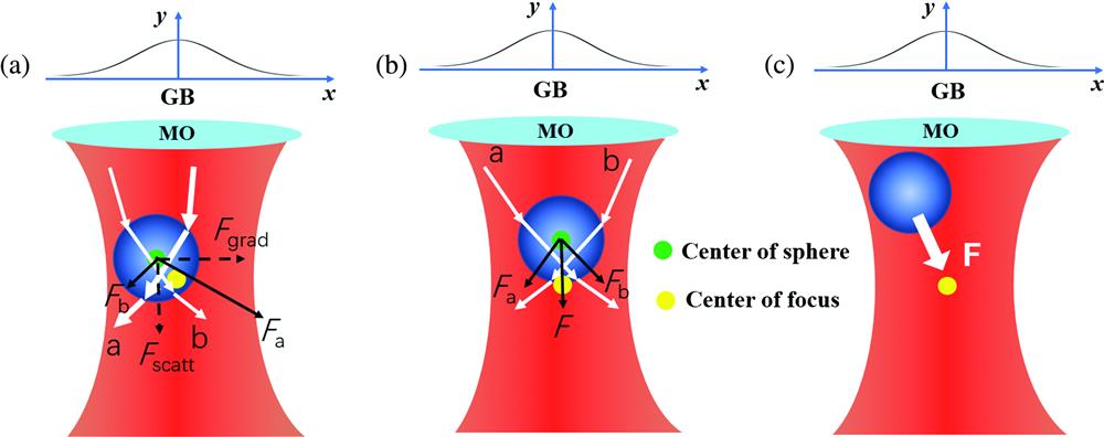
First, we use the simple ray optics model to explain how optical tweezers work. Figure 1(a) shows a laser beam with two light rays (white arrows a and b) passing through a dielectric spherical particle located off-axis of the laser beam. The light rays will change their propagation directions due to the refraction, resulting in a change in their momentum. As shown in Fig. 1(a), the central portion of the beam with higher intensity (indicated by a thick arrow a) is refracted to the left, which means a change in the laser’s momentum to the left. Based on the conservation of momentum at the particle boundary, the particle will feel a momentum kick to the right and therefore has a force toward the center of the beam (dotted line). Analogously, the light ray b with lower intensity will change its momentum to the right and exert an optical force on the particle away from the beam center. Since the light ray represented by a is much stronger than the ray represented by b, the net force will push the particle to the right. Conversely, if the particle is located on the right side of the beam axis, the optical force will push it to the left. As such, the light field intensity gradient always causes a gradient force () on the particle toward the maximum intensity of the beam. Besides, the rays reflected from the particle surface can produce forward scattering forces () along the beam propagation direction. Figure 1(b) shows the longitudinal gradient force pushing the particle down toward the focal plane, and vice versa, in a highly focused laser beam. Therefore, the net force pushes the particle to the focus of the beam, as shown in Fig. 1(c). In the case of , a stable 3D trap can be formed in a tightly focused laser beam spot.
Figure 1.Schematic diagram of optical tweezers: (a) when the particle is away from the center of the beam focus, (b) when the particle is slightly above the center of the beam focus, and (c) net force acting on the dielectric sphere. and are the forces produced by the refracted rays a and b, respectively. and denote the gradient force and scattering force, respectively. GB, Gaussian beam; MO, microscope objective.
In the Rayleigh regime, ray optics are not applicable to explain the optical forces, as the particle size is smaller than the wavelength of light. Here, the particle needs to be considered as a point electric dipole, and the optical forces can be written as42where is the polarizability of the particle, and , are the electric field and magnetic field, respectively. denotes the total particle cross-section. The first term in Eq. (1) indicates the gradient force (), and the last two terms represent the scattering force (). The second term in Eq. (1) is normally called the scattering force, and the third term is the so-called spin curl force.42
Equation (1) indicates that each of these three optical forces on a particle depends on the polarizability, which can be expressed as42where is the Clausius–Mossotti relation, is the particle radius, and is the relative refractive index of the particle to the surrounding medium. Therefore, we can play with the polarizability to optimize the optical traps. Then, the optical gradient force and optical scattering force can be rewritten as2,43and where is the speed of light, is the unit vector along the direction, is the intensity of light, and is the wavenumber.
Both the ray optics and the dipole theory are powerful tools to study the optical forces in their respective size regimes, which have all given good physical pictures of the trapping mechanism. However, particles with their size lying between these two regimes make these approaches no longer valid. Instead, the Lorenz–Mie theory can be used to calculate the optical forces for such particle sizes, which are the exact solutions of the Helmholtz equations.41,44 If the particles are not spherical, or the incident beam is not a plane wave, the generalized Lorenz–Mie theory can be used.45 There are also many other fully numerical methods to calculate the optical force, such as finite-difference time-domain (FDTD) and finite element method. For instance, the FDTD analysis allows the numerical simulation of the scattered light field over an arbitrary particle. The optical force would be the surface integral of the Maxwell stress tensor. It should be noted that nondielectric materials, e.g., metals, semiconductors, and nonspherical particles, require different approaches. Proper choice of the force evaluation method relies on particle size, geometry, and the structure of the light field.45,46
A conventional optical tweezers system is schematically shown in Fig. 2. First, a collimated laser beam is expanded to overfill the back aperture of a microscope objective. A dichroic mirror () reflects the laser beam to the high numerical aperture (NA) objective lens, which focuses the beam to a tightly focused diffraction limited spot inside a sample chamber for trapping. To image trapped particles on a CCD camera through , an LED white light source is typically used to illuminate the sample. A condenser lens collects forward scattered light from the trapped particles and projects an image onto a quadrant photodetector (QPD) using back focal plane interferometry.34 The balanced photodetection provided by the QPD allows the precise measurement of the motion of the trapped particles. The axial position can be measured by the sum of the intensity of the four quadrants.34
Figure 2.Experimental configuration of conventional optical tweezers. A simple telescope is used to expand the laser beam to overfill the back aperture of the objective. The expanded laser beam, reflected by a dichroic mirror (), is coupled into the objective. The laser beam is focused by the objective and forms an optical trap. The QPD is placed in a conjugate plane of the condenser, to collect the forward scattered light that is reflected by the dichroic mirror (). The trapped particles are imaged with a CCD camera. The lateral () position of the particle can be measured by the normalized output voltage signals from the four quadrants, namely, and .
The motion of a Brownian particle in a fluid can be described by the Langevin equation.47 In the overdamped case, where particles are immersed in a viscous medium, e.g., water, the one-dimensional motion ( direction) of an optically trapped Brownian particle will be described by the equation where the thermal random force drives the Brownian motion through collisions with surrounding molecules of the fluid, and is the Stokes drag coefficient ( is the viscosity of the fluid, and is the radius of the particle). The trap stiffness , where is the mass of the particle, and is the trap frequency, determines the magnitude of the optical restoring force depending on its position relative to the trap center. For a silica particle of radius () in water at room temperature, the resonant frequency of the harmonic oscillator is for typical stiffnesses in the range of .
The power spectral density (PSD) of the particle’s motion can be used to characterize the trap. At equilibrium, the PSD is Lorentzian.48 For the particle’s displacement, where is the corner or roll-off frequency that verifies the trap stiffness. The integral of the PSD in units of yields the position variance or the mean square displacement (MSD) of the particle, which verifies the equilibrium temperature of the particle: The position variance directly measured by a CCD or a QPD (see Sec. 2.1) can also verify the trap stiffness, which benchmarks the PSD method.
2.3 Optical Torques for Rotation
Rotation of micro- and nano-objects, caused by the transfer of angular momentum from light beams, is of great interest due to its potential applications in optically driven micromachines, motors, actuators, or biological specimen. A beam of circularly polarized light carries spin angular momentum (SAM), which was derived by Poynting49 in the early 1900s. The first experimental observation of SAM was performed by Beth50 in 1936. In this experiment, he observed a mechanical torque on a double refracting slab due to a change in the circular polarization based on the conservation of angular momentum. It is now well understood that SAM of per photon is associated with the circular polarization of light, where the sign depends on its handedness. SAM of light has been used for rotation of both elongated, birefringent, and absorbing particles as well as particle cluster in optical tweezers.34 Notably, with birefringent particles,51 a maximal torque efficiency of per photon can be achieved, contrary to the per photon achieved with elongated particles. In addition, optically trapped micron-sized birefringent particles were rotated by a circularly polarized beam at rotating rates as high as 350 Hz in water39 and 10 MHz in vacuum.40 Crucially, in recent time, it was demonstrated that SAM can also be used for the selective 3D trapping of chiral micro- and nanoparticles.52,53 It was shown that under appropriate conditions, a light beam with SAM can induce nonrestoring or restoring forces on chiral microparticles.52 Similar results have been also reported on the interaction of chiral nanoparticles with chiral optical fields.53
In 1992, Allen et al.25 introduced the concept of a light beam possessing OAM, which is in addition to any SAM and characterized by an azimuthally varying phase of , where is an integer value, termed the topological charge, and is the azimuthal angle. The first experimental demonstration of OAM transfer from light to matter, in the context of optical tweezers, was performed by the group of Rubinsztein–Dunlop,54,55 who demonstrated the optically induced rotation of absorptive particles. This was followed by the demonstration of the simultaneous transfer of both SAM and OAM to the same absorptive particles with circularly polarized modes.56 In these experiments, the rotation rate was shown to be proportional to the sum of SAM and OAM, i.e., the total angular momentum.57 Other pioneering experiments include the transfer of SAM and OAM to a birefringent particle, which causes the particle to spin about its own axis as well as to rotate about the beam axis,58,59 as shown in Fig. 3. While these previous demonstrations were performed with particles confined in two-dimensions, with the particle being pushed against a microscope slide, a key experiment that demonstrated the transfer of SAM and OAM to particles in 3D was performed by Simpson et al.60 Besides the high-index particles, the 3D optical trapping of low-index particles has been studied as well,61,62 and it was shown that the low-index particles can be trapped stably on the axis and slightly above the focal plane of a strongly focused optical vortex beam.
Figure 3.Optical trapping of birefringent microparticles that show the transfer of OAM and SAM. (a) The trapped particle is spinning counterclockwise about its own axis (left column) and orbiting clockwise about the beam’s axis (right column) separately. Adapted from Ref. 58. (b) The particle rotates around its own axis (left column) and the beam’s axis (right column) simultaneously. Adapted from Ref. 59.
Light is an electromagnetic wave; as such, it can be characterized by its wavelength (color), amplitude, and phase or polarization, the later associated with the direction of oscillation of the electromagnetic field in space, transverse to the direction of propagation. For unpolarized light, the direction of oscillation is random. On the contrary, for polarized light, this can take distinctive forms including linear, circular, or elliptical, which are the preferred configurations for beam shaping. In what follows, we will restrict our review to the case of polarized light, first discussing the case of homogeneous polarization (scalar fields), followed by the nonhomogeneous case (vector beams). Inevitably, any discussion about structured light fields involves the Helmholtz equation, either in its exact or paraxial forms. As such, we will start our discussion by reviewing some of the most relevant solutions to the Helmholtz equation that have played a crucial role in the development of optical tweezers with structured light as we know them today.
3.1 Laguerre–Gaussian Beams
Laguerre–Gaussian (LG) modes are a set of solutions to the paraxial wave equation in cylindrical coordinates. Their normalized transverse profile can be defined as25where () is the associated Laguerre polynomials with and as the azimuthal and radial indices, respectively. A set of the parameters , , and is defined as , , and , respectively. Here, is the Rayleigh range, and is the beam waist. Importantly, LG beams carry OAM per photon, associated with the phase term . This phase term results in a spiral azimuthal phase that creates an inclined wavefront. The Poynting vector has, therefore, a nonzero azimuthal component that is at the origin of the angular momentum. Figure 4 shows four examples of the transverse intensity profiles of LG modes.
Figure 4.Transverse intensity profiles of LG modes with (a) , (b) , (c) , and (d) . The color denotes the normalized intensity distribution.
Another set of solutions to the Helmholtz equation in free space, when solved in cylindrical coordinates , is the Bessel modes,63–65where represents the ’th order Bessel polynomial, and is associated with OAM per photon carried by the beam. Moreover, and are the transverse and longitudinal components of the wave vector , respectively, obeying the relations and .
A more intuitive way of describing a Bessel beam is by considering these as the result of a superposition of plane waves propagating on a cone, where each of them undergoes identical phase shifts, over a distance . This interpretation can be observed in the angular spectrum of the Bessel beam, which takes the form of a ring or radius in the -space. Therefore, the optical Fourier transform of the Bessel beams is a ring, and, vice versa, the optical Fourier transform of a ring will result in a Bessel beam. Therefore, Bessel beams can be generated using a ring-slit aperture.64 Using this method, Durnin63 produced a Bessel beam experimentally for the first time. Figure 5 shows this concept schematically; in Fig. 5(a), we show the transverse intensity profiles of a Bessel beam with topological charge and its Fourier transform, while in Fig. 5(b) we show that of a Bessel beam of topological charge along with its Fourier transform.
Figure 5.Transverse intensity profiles of Bessel beams and its Fourier transform with (a) and (b) . The color denotes the normalized intensity distribution.
Two of the most prominent properties of Bessel modes are, on one hand, their tendency to maintain an invariant intensity profile, namely, and, on the other, their tendency to recover its original form when an opaque obstruction is placed in its path.64 Such a property can be explained by invoking again the plane waves propagating on a cone approach as detailed next. When the opaque object or radius is placed in the center of the Bessel beam, some of the waves that create the beam are blocked by this object, creating a shadow region. Nonetheless, some other plane waves can pass the object unaffected, which ultimately are the ones that reconstruct the intensity profile of the beam after a certain propagation distance.65,66 As mentioned earlier, Bessel beams can be generated by placing a slit aperture in front of a ring-slit aperture; none the less, this is a very inefficient way since most of incident beam’s intensity is blocked. A far more efficient way to produce a Bessel beam is using an axicon.64 The on-axis intensity is formed by conical wavevectors that propagate on the surface of a cone.
As we will discuss later, the zeroth-order Bessel beam has demonstrated its great relevance in optical trapping for the study of multiparticle arrangements along the beam axis.67,68 Since Eq. (9) shows that these modes have infinitely extending sidelobes and carry an infinite amount of energy, their experimental realization is approximated by adding a Gaussian envelope. These modes are known as Bessel–Gauss modes, which at take the form69,70
3.3 Perfect Vortex Beams
The concept of the “perfect vortex beam” was proposed by Ostrovsky et al.,71 whose intensity profile is independent of its topological charge. Its complex amplitude at a given propagation distance can be expressed as71where is the radius of the bright ring, is the width of the ring, and, in general, . Contrary to LG modes, in which the radius of the ring-like transverse intensity profile scales up with the topological charge, in perfect vortex modes, it remains constant. Even so, recent reports suggest that the width of such modes experiences a small scaling with the topological charge.72 This is shown in Fig. 6, where the transverse intensity profiles of a set of perfect vortex beams with topological charges , 4, 10, and 15 are shown. Vaity and Rusch73 pointed out that a perfect vortex beam is actually a Fourier transform of a Bessel beam, and it can be generated by employing a phase hologram whose transmittance is the phase of a Bessel beam.71–74 It is worth noting that although the concept of “perfect vortex beam” was proposed in 2013, such a beam had been introduced and used for 3D optical trapping and transport of particles by Roichman and Grier,75 Roichman et al.76 had pointed out that the radius of this 3D ring trap is independent of the topological charge, and the first experimental demonstration of optical trapping using the “perfect vortex beam” has been reported under the name holographic ring trap. The perfect vortex has been used by the optical trapping community as a particular case of the structured light beam to study the dynamics of driven particles in the form of optical matter.77–80
Figure 6.Transverse intensity distribution of perfect vortex beams with topological charge , 4, 10, and 15. Here, is the radius of the ring-like intensity profile and its width. Notice that the intensity profile remains constant as increases. The color represents the normalized intensity distribution.
Another interesting set of vector modes is the Mathieu–Gauss beams, which are obtained when the Helmholtz equation is solved in elliptical cylindrical coordinates.59 In such coordinates, defined by , , and , where is the radial coordinate, and is the angular coordinate, the Helmholtz equation can be separated into a longitudinal part and a transverse part. The former is easily solved by having a solution of the form , and the latter is found as a solution of the equation81,82
Here, the semifocal distance is represented by , given in terms of the major and minor as rand , and related to the eccentricity as . Further, the parameter is the transverse component of the wave vector . Equation (12) can be split into the radial and angular Mathieu equations, using the well-known separation of variables technique to obtain the nondiffracting Mathieu beams:83
In the above, and are normalization constants, whereas and are the even and odd radial Mathieu functions, respectively, and and are the even and odd angular Mathieu functions. For even modes, the subindex , while for odd modes it takes the values . Again, the nondiffracting Mathieu beams carry an infinite amount of energy and cannot be realized experimentally. Nonetheless, a finite-energy version can be realized using a Gaussian envelope, which is known as the Mathieu–Gauss beam. Such modes retain the nondiffracting properties of the ideal Mathieu beams over a finite propagation distance. The Mathieu–Gauss modes are described mathematically as83
Using the new definitions, and , where now is the semifocal separation at . The parameter is defined in terms of the Rayleigh range as, , where is the waist radius of a Gaussian beam. Figure 7(a) shows the transverse intensity distribution of a set of even, while Fig. 7(b) shows those of odd Mathieu–Gauss beams, given by the parameters , , , and . Importantly, Mathieu–Gauss beams are another class of “nondiffracting” optical fields, which are a variant of superposition of uniform conical waves, i.e., Bessel beams. Therefore, they have a similar capability of self-reconstruction after an opaque finite obstruction.
Figure 7.Transverse intensity pattern of a truncated zeroth-order Mathieu beam with (a) even and (b) odd modes. The color represents the normalized intensity distribution.
Another important solution to the paraxial wave equation is the Airy beam, which is given in ,84,85where and are dimensionless coordinates in the transverse plane and set by the scale parameters and . Moreover, represents a normalized propagation distance. Similar to the Bessel modes, Airy beams exhibit unique properties of self-acceleration, “nondiffraction,” and self-reconstruction. Among these, its tendency to accelerate in the transverse plane following a parabolic trajectory has attracted considerable interest [see Figs. 8(a) and 8(b)]. Since Airy beams also carry an infinite amount of energy, its experimental realization with finite-energy can be approximated by Airy–Gaussian modes [see Figs. 8(c) and 8(d)] and given as where is a negative parameter that limits the energy of the Airy beam. As a result, the nondiffracting property can only persist for a finite distance. The inverse Fourier transform of at yields a product of a Gaussian beam and a cubic phase,84where and are the transverse components of the inverse Fourier transform. Therefore, we can experimentally generate an Airy beam by modulating a Gaussian beam with a cubic phase in the Fourier domain.
Figure 8.Airy beam profiles. (a) Parabolic trajectory and (b) transverse intensity profile of an Airy beam with infinite energy compared with those of a finite energy Airy beam in (c) and (d). The color represents the normalized intensity distribution.
The Ince–Gaussian (IG) modes are another important family of orthogonal solutions to the paraxial wave equation, which can be described as86,87where and represent the even and odd solutions of order and degree , with and being normalization constants, and and being even and odd Ince polynomials, respectively. together with , are the scale parameters related to the geometric size of the mode. We note that IG modes are a continuous transition from LG to Hermite–Gaussian modes. Figure 9 shows the intensity profiles of even [Fig. 9(a)] and odd [Fig. 9(b)] IG modes for .
Figure 9.Transverse intensity distribution of low-order (a) even and (b) odd IG modes with , , and . The color represents the normalized intensity distribution.
Helico-conical (HC) beams, contrary to the above optical modes, have radial phase dependence.88,89 The phase in HC beams is unique, and it is given by a product of both the radial and the azimuthal coordinates,66where is the topological charge, is either 0 or 1, and is a normalization constant in the radial coordinates. As a result of this phase dependence, upon propagation, the optical field exhibits a helical geometry with anomalies in both phase and amplitude. Figure 10 shows the transverse intensity profiles of the HC beam comparing experimental and simulation results. Interestingly, these beams also exhibit a self-healing property, as demonstrated recently.67
Figure 10.Intensity distribution of an HC beam from numerical simulations. (a), (c) The near-field intensity distribution; (b), (d) the far-field. (a), (b) ; (c), (d) . In all cases, . The color represents the normalized intensity distribution.
In the previous sections, we considered a set of structured light fields, in which the polarization distribution in the transverse plane was homogeneous. Here, we will now look into a more general class of light fields with spatially inhomogeneous polarization, commonly known as vector beams, which arise naturally as solutions to the vectorial Helmholtz equation.90,91 These modes are commonly regarded as nonseparable superpositions of spatial modes and polarization,92where the spatial degree of freedom is represented by the orthogonal functions and , and the polarization degree of freedom is represented by the orthogonal unitary vectors and in the circular polarization basis. Moreover, the parameters and are intermodal phases that introduce a phase delay between both polarization components. Note that the spatial degree of freedom spans an infinite space, and the number of combinations between the spatial and polarization degrees of freedom is also infinite, giving rise to an infinite set of vector modes. In principle, the spatial degree of freedom can be any of the scalar modes described above. In the basis, Eq. (23) can be rewritten as91,92
In principle, and can take any integer value. Here, we will consider the simplified case of , and , , in which case, Eq. (24) can be expressed as
By substituting , the following set of orthogonal vector modes can be obtained:
These cylindrical vector modes are commonly known as Bell states, which are eigenmodes of both free-space and optical fibers.93 Both the and modes with radial [Fig. 11(a)] and azimuthal [Fig. 11(c)] polarizations have been used in optical tweezers due to their unique transverse and longitudinal force components in the trapping plane. This will be discussed in more detail in a later section.
Figure 11.Intensity and polarization distribution of the fundamental cylindrical vector beams. (a) Radial, (b) hybrid odd, (c) azimuthal, and (d) hybrid even modes. The color represents the normalized intensity distribution, while the lines are associated with the polarization orientation of the electric field.
Experimentally, the complex beams described above can be generated in a wide variety of ways, which include interferometric arrays,94–96 glass cones,97,98 liquid crystal wave plates,99,100 metamaterials,101 spatial light modulators (SLMs),102–105 and, in recent time, digital micromirror devices (DMDs).106–108 Noteworthily, SLMs enable the generation of complex 2D and 3D shaped light beam patterns, which have significantly advanced the configurable optical trapping of particles. Since these devices are typically utilized in the Fourier plane of an optical system, optical trapping systems using holographically generated light beams are known as holographic optical tweezers (HOTs). In this section, we overview the use of complex light fields in optical tweezers.
4.1 Optical Trapping with Propagation Invariant Beams
In this section, we will discuss some of the key demonstrations of HOTs within the domain of single optical traps.
4.1.1 Optical tweezers with Laguerre–Gaussian beams
As discussed in Sec. 2.2, the LG beam is one of the most common beams used for optical trapping. Since the high-order LG beams can carry OAM, which can be used to achieve the orbital rotation of particles. Pioneering experiments demonstrated a full 3D rotational control of microspheres and biological specimens using modes.109,110 The modes were interferometrically combined with a reference mode (Gaussian mode) to produce a spiral structure. While the phase profile of the mode can be considered to be flat (spherical more precisely), the modes are featured with a more intricate structure, resembling a helical staircase. Hence, the interference of an mode with a Gaussian mode produces a new structured azimuthal phase with an intensity pattern containing spiral arms. Importantly, the spiral structure can be rotated in any direction and at arbitrary rates by introducing phase delays in one of the arms of the interferometer. In this way, particles trapped in the bright lobes of the interference pattern can be rotated in any direction around the optical axis of the beam. By simply changing the azimuthal index , it is possible to manipulate objects with different shapes or to trap many objects simultaneously.109 Importantly, this pioneering experiment showed for the first time the potential application for the control of biological organisms, in which case, the authors trapped and rotated a Chinese hamster chromosome.
Another experiment110 was performed using a collinear interferometric superposition of modes, with opposite topological charges and , to produce the intensity patterns with petal-like structures of bright lobes. Similarly, the structure could be rotated by introducing phase delays in one of the arms. Figures 12(a) and 12(b) show 3D manipulation and rotation of particles trapped in intensity patterns produced by the superposition of and . Figure 12(c) shows the rotation of the 3D microstructure of particles. Finally, Fig. 12(d) shows a schematic representation of the 3D structures that were created in this experiment by stacking more particles on each bright spot.
Figure 12.Optical trapping and control of 3D structures using superpositions of and as the trapping beam. (a) Two microspheres trapped at the two bright spots created by the superposition of the modes and . (b) Trapping and release of eight microspheres trapped along the beam’s propagation axis by the intensity pattern generated by superposed modes of and , as schematically shown in (d). (c) Rotation of the eight-microsphere cubic structure. (e) Schematic representation of the generation of 3D structures containing a larger number of microspheres. Adapted from Ref. 110.
More recently, LG beams were used to explore the manipulation of single or multiple silicon nanowires.111 It demonstrated the orbiting of silicon nanowires around the optical vortex aligned parallel to the propagation axis of the beams. Figure 13(a) shows the position of the particles as a function of time, evincing a clear orbital motion; the right inset shows a schematic representation of the trapped nanowire overlapped with the intensity pattern of the trapping beam. In addition, the author demonstrated that silicon nanorods oriented perpendicular to the propagation axis of the beam can be used as light-driven nanorotors, resulting from the transfer of SAM.
Figure 13.Optical trapping and rotations in counterpropagating circularly polarized LG beams of silicon nanowires aligned (a) parallel and (b) perpendicular to the beam propagation axis, where orbiting and orbiting-reorientation are shown, respectively. The simultaneous spinning and orbiting of a shorter nanowire is shown in (c) and (d). Adapted from Ref. 111.
It is noted that the small particles can be trapped in the bright ring of LG vortex beams, while if the size of the particle is comparable to the waist size of the incident structured beam, the particle is predicted to be trapped at the center of the beam with the proper choice of the beam parameters such as vortex charge and polarization.112 Moreover, a very recent study showed that when the LG beam is strongly focused, the rotation direction of the trapped particles might be in the opposite direction,113 which is much different for the case of paraxial LG beams. Figure 14 shows the anomalous motion of a particle trapped in a strongly focused LG beam. From Fig. 14(c), we can see that in the region , the direction of the optical torque is opposite that of OAM of the LG beam.
Figure 14.Anomalous motion of a particle trapped in strongly focused high-order LG beams. (a) The intensity profile of the LG beam with topological charge 3. (b) The plot of the distribution of the radiation force exerted on the trapped particle for different center-of-mass radii. (c) The radial (blue line) and azimuthal (red broken line) components of the radiation force for different radii of the trapped particles. Adapted from Ref. 113.
The trapping geometry and particle shape can have a great influence on the angular momentum transfer. Jesacher et al.114 reported an observation of particles orbiting in a reverse direction with respect to the OAM of the incident light field. Irregular-shaped glass microparticles were trapped at an air–water interface with an LG mode of topological charge based on the holographic tweezers setup. Figure 15 shows the rotation of a polystyrene bead and a glass sliver depending on the sign of the topological charge. Intriguingly, only the polystyrene bead changes its direction of rotation by inverting the topological charge.
Figure 15.Rotation of a polystyrene bead and a glass sliver trapped with an LG mode of . (a) Sequential images of these particles showing their direction of rotation. (b) Angular velocity of each particle with respect to the topological charge. Adapted from Ref. 114.
A simple ray optics model for a wedge-shaped glass particle placed at the air–water interface indicates that reflection and refraction of light rays on the particle surfaces can cause the asymmetric object to move against the direction of the OAM of the incident light field. Importantly, this demonstration suggests that the shape-anisotropy of the particles could be optimized for optical momentum transfer and thus for efficient optical nanotransport techniques. Other demonstrations of negative optical torques include reversed orbiting and spinning with a Bessel light beam,115 elliptically polarized beams,116 and circularly polarized Gaussian light beams.117
4.1.2 Optical trapping with Bessel–Gaussian beams
With the nondiffracting property, Bessel beams have great advantages for optical manipulation. The first experiment using zeroth-order Bessel beams demonstrated the trapping of multiple particles along the beam axis, as well as the transport of these particles over long distances ().26 Subsequent experiments68 showed the manipulation of microparticles in multiple optical planes along the beam axis, using two sample cells ( in thickness) separated by 3 mm, as shown in Fig. 16(a). Crucially, even though the Bessel–Gaussian beam is distorted by the particles in the first cell, its self-healing properties allow recovery of its original intensity profile after a certain propagation distance, which coincides with the separation distance of the cells. Hence, the beam is capable of trapping again microparticles in its multiple rings inside the second cell. We note that in this experiment, the radius and nondiffracting propagation distance of the Bessel–Gaussian beam are and , respectively. It is worth mentioning that such a beam can also align multiple rods along the beam propagation direction.68 Along the same line, counterpropagating Bessel beams have also been used to manipulate submicron particles in three dimensions. This optical conveyor belt is based on the generation of a standing wave, created from the on-axis superposition of two counterpropagating Bessel beams, which allows us to confine and deliver over long distances (hundreds of micrometers) and with high precision multiple submicron particles [Fig. 16(b)]. The delivering of particles was achieved by dynamically changing the phase of one of the beams, which in turn causes the whole structure of nodes and antinodes to shift along the optical axis of the standing wave.118 In 2008, a practical application was demonstrated, where microspheres trapped with Bessel beams served as objective lenses to focus a laser onto a surface to enable near-field direct writing with nanometer resolution.119 This technique was used to demonstrate nanopatterning of arbitrary patterns with dimensions in the order of 100 nm and positioning accuracy in the order of 40 nm.
Figure 16.Optical trapping with Bessel beams. (a) Trapping of multiple particles at different optical planes. Adapted from Ref. 68. (b) Trapping and delivering of two particles using a sliding Bessel standing beam. Adapted from Ref. 118.
Very recently, a superposition of multiple copropagating Bessel beams, so-called frozen waves, was used to build stable optical trapping as well.120 Besides demonstrating that such beams possess greater optical trapping stabilities, the authors also demonstrated their capabilities of trapping in multiple parallel planes along the propagation direction, as schematically shown in Fig. 17(a). Here, to observe the motion along the propagation direction, the authors implemented a digital propagation, in which the observation plane is fixed, and different propagation planes are simulated holographically by changing the hologram that generates the frozen waves. An experimental sequence of frames of the beam at different propagation planes is shown in Figs. 17(a1)–17(d1) and 17(a2)–17(d2) for the case on one and two trapped particles, respectively.
Figure 17.(a) Schematic representation of optical trapping with frozen waves in multiple parallel planes. Sequence of (a1)–(d1) one and (a2)–(d2) two microparticles (orange circle) trapped at different transverse planes along the propagation direction. Adapted from Ref. 120.
If we replace the zeroth-order Bessel beams with higher-order Bessel beams, namely, Bessel vortex beams, the situation will change significantly. That is because the center of the Bessel vortex beam has zero intensity, due to the phase singularity on the axis. Therefore, the trapping of multiple transparent particles in multiple rings of intensity maxima of higher-order Bessel beams was experimentally demonstrated,70 and the rotation of the trapped particles is observed as well. It is worth noting that the optical trapping behavior is dependent on the size of the particles.121 If the size of the particle is much smaller than the radius of the vortex bright ring, the particle will be trapped in the bright ring; meanwhile, the trapped particle will orbit along the bright ring, as shown in Fig. 18(a). If the size of the particle increases and is close to the radius of the vortex ring, then the particle will be trapped stably, without rotation, at certain off-axis positions of the inner bright ring, as shown in Fig. 18(b). If the particle is large enough to cover the whole bright ring of the vortex beam, then the particle will be trapped in the center of the vortex beam, and the particle does not rotate [Fig. 18(c)]. As a comparison, Fig. 18(d) shows the optical trapping of a silver nanowire with an LG vortex beam, and it was shown that the nanowire rotates only if its length is longer than the size of the bright ring of vortex beam.122
Figure 18.Effect of the size of the trapped particle on optical trapping with vortex beams. (a)–(c) Optical forces of a particle with different sizes compared to the radius of the bright rings of Bessel vortex beams. The blue circle and blue dot denote the edge and the center of the trapped particle. The cyan contour denotes the zero force azimuthal directions. The magenta lines represent the deterministic trajectory of a particle. (d) Illustration of a rotation of a single silver nanowire trapped by an LG vortex beam. (a)–(c) Adapted from Ref. 121. (d) Adapted from Ref. 122.
Optical manipulation using perfect vortex modes possessing annular intensity profiles independent of topological charges has been of great interest in recent years.123 The motion of trapped particles is determined by the gradient and scattering forces resulting from the perfect vortex beam. The particles continuously move along the annulus due to the scattering force from the inclined wavefront, as shown in Figs. 19(a) and 19(b). As the OAM density is well-defined in the perfect vortex beam, a linear relationship between the rotation rate and the OAM is guaranteed for both negative and positive topological charges, as shown in Fig. 19(c). The experimental realization of perfect vortex beams is rather challenging, as they tend to exhibit azimuthal intensity variations due to optical aberrations. As a result, the rotation of a single particle is difficult to maintain at a constant velocity around the trap due to local intensity hot spots. Nonetheless, with intensity profile correction techniques, it is possible to eliminate these hot spots,123 in which a single trapped particle can continuously move along the vortex ring, as schematically illustrated in Fig. 19(d). However, the trapped particle still exhibits a nonuniform angular velocity due to local variations of the OAM density,124 as shown in Fig. 19(e). Based on the linear dependence of the particle rotation rate upon the OAM density, the angular velocity can be adjusted in situ by correcting the local OAM density with a phase correction mask. It is worth noting that experimentally the perfect vortex beam can induce rotation of the trapped particle at a constant velocity with integer topological charges, while fundamentally this cannot be achieved with fractional topological charges.74
Figure 19.(a) A perfect vortex beam with and (b) the beam with the scattered light from a single trapped particle. (c) Linear relationship between the particle rotation rate and the integer topological charge. (d) Snapshot of a trapped particle rotating around the circumference of a perfect vortex beam indicated by the red circle. (e) Angular velocity of the particle as a function of its angular position. Adapted from Refs. 123 and 124.
Mathieu beams are a family of propagation invariant beams with self-healing properties. Compared to Bessel–Gaussian beams, they are especially well-suited for the 3D arrangement of particles due to their rich variety of complex transverse mode distributions.125 Notably, Mathieu beams allow us to trap and orient elongated objects in the transverse plane to the beam () axis, which is not normally possible with single optical tweezers. Figure 20 shows optical trapping of nonspherical particles with a fourth order () even Mathieu beam [Figs. 20(a)–20(c)], which was rotated within the plane [Figs. 20(d) and 20(e)]. Elongated particles () were arranged with their long axis in the transversal plane [Figs. 20(f) and 20(g)], and their orientation depends on the beam orientation.
Figure 20.Optical trapping of nonspherical particles. (a) Mathieu beam with . (b) 3D intensity distribution. (c) Particles orientation within transversal intensity distribution. (d) Rotating hologram and (e) corresponding Mathieu beam. (f) Time-lapse images of trapped particles depending on the orientation of the Mathieu beam and (g) their corresponding schematics. Adapted from Ref. 125.
We note that it is possible to assemble multiple particles in the direction because of the self-healing property of Mathieu beams. Furthermore, Mathieu beams also offer superpositions of even and odd modes, resulting in helical Mathieu beams that provide continuous phase variations. Thus, these beams were also used to investigate the transfer of OAM126 to particles in optical micromanipulation.127
4.1.5 Optical trapping with Airy–Gaussian beams
One of the most prominent properties of Airy beams is their ability to freely accelerate in the transverse plane, resulting in a parabolic trajectory upon propagation. Exploiting this property, Baumgartl et al. transported particles along parabolic trajectories, as schematically represented in Fig. 21(a).128,129 An Airy beam was shaped from a 25-mW argon-ion laser using an SLM and focused down to a size of into a chamber containing an aqueous suspension of colloidal glass microspheres. The optical gradient forces attracted particles toward the main lobe of the Airy beam, where they were transported along the parabolic trajectory due to radiation pressure. The Airy beam shifted laterally over a distance of after only a propagation distance of . Figures 21(b) and 21(c) show experimental results of the so-called “snowblowing” effect. The field of view was divided in four quadrants marked with different colors to see this effect clearly. Figure 21(b) shows that an Airy beam launched into the second (green) quadrant cleared particles in this section by carrying them into the third (purple) quadrant along the 3D parabolic trajectory. This process is reversible if the orientation of the Airy beam is inverted, as shown in Fig. 21(c). Recently, a circular Airy vortex beam has attracted interest due to its autofocusing property,130,131 which is a hollow beam carrying OAM, as shown in Fig. 21(d). Such a beam carries OAM, which can be used to trap and rotate particles as well, as shown in Fig. 21(e). Moreover, it is shown that the rotational velocity of the trapped microparticles first increases with the increasing topological charge and then decreases after it reaches a maximum.130
Figure 21.Optical manipulation with Airy beams. (a) Schematic representation of a microparticle being transported along a parabolic trajectory. Adapted from Ref. 128. Transporting particles (b) from quadrant two (green) to quadrant three (purple) and (c) from quadrant three to quadrant two. Adapted from Ref. 129. (d) The plane intensity profile of a circular Airy vortex beam. (e) Rotation of the trapped silica particles on the primary ring of circular Airy vortex beam for topological charge 12. The white and yellow circles denote the vortex ring position and the position of a selected trapped particle at different time. Adapted from Ref. 130.
As previously mentioned, IG modes appear as natural solutions to the paraxial wave equation in elliptical coordinates (see the previous section on IG modes). A rich variety of transverse intensity profiles given by high-order assemblies of this family of modes allow micromanipulation of particles at each bright spot. Woerdemann et al.132 utilized these IG modes to create 3D structures of trapped microparticles. Figure 22 shows the IG modes generated by an SLM (top row) and particles trapped in the bright parts of these IG modes (bottom row). Notably, microbeads can be trapped in 3D according to the 3D structures of these beam profiles.
Figure 22.Micromanipulation with IG beams. The top row shows the transverse intensity patterns of the beams, while the bottom row shows trapped microparticles with the corresponding beams. (a) mode. (b) mode with four columns of particles stacked along its beam axis. (c) mode where the four central petals close to each other show no stable traps. (d) mode with particles trapped at certain locations. Adapted from Ref. 132.
Another important class of OAM beams is the HC beams with spiral phase and intensity profiles.88,89 A schematic representation of beam generation and its 3D beam profile upon propagation are shown in Fig. 23(a). With this unique beam property, both linear momentum and OAM are to be transferred to microparticles.133 In the experiment, -diameter silica beads are dispersed in water in a chamber with a thickness of . Figure 23(b) shows time-lapse images of a trapped bead moving upward from the bottom along a spiral trajectory around the axis of the HC beam ().
Figure 23.Optical manipulation with HC beams. (a) Schematic representation of the setup required for beam generation. (b) Time-lapse images of a microbead trapped and guided along with the maximum intensity of the beam, as illustrated on the left. Adapted from Ref. 133.
4.2 Optical Trapping with Holographic Optical Traps
4.2.1 Holographic arrays of multiple optical traps in two and three dimensions
As we have shown in previous sections, SLMs have provided the ability to create 2D and 3D optical traps for guiding or transporting microparticles. Nonetheless, most of the previously discussed techniques rely on the use of common light beams that are solutions to the wave equation, except for HC light beams. In what follows, we will discuss a more general class of optical traps, which rely on arbitrary customized 2D and 3D light beams.
An immediate and almost obvious step forward to achieve the simultaneous trapping of many particles is through the use of galvo-scanning mirrors or acousto-optic beam deflectors,134 in which a single beam can be time-shared at multiple locations to simultaneously trap micron-sized polymer spheres. This approach can be used in the study of the single molecule H-NS protein, for example.134 An alternative approach to generate arrays of optical traps relies on the use of diffractive optical elements (DOEs),135 as shown in Fig. 24. The key idea in this approach is based on the deflection of an input beam to a different angle defined by period of a diffraction grating. Therefore, the generation of multiple trapping focal spots can be achieved by superimposing multiple diffraction gratings. A typical binary version of the DOE pattern for a hexagonal tweezers array is shown in Fig. 24(b). The trapped microspheres in the array are shown in Fig. 24(c).
Figure 24.Optical tweezer arrays using computer-generated holograms. (a) Schematic representation of the fields at the input hologram and output Fourier planes, where is the wave vector. (b) DOE (the black color represents a phase shift of -rad) etched on a fused silica substrate for a hexagonal array of traps. (c) 19 silica spheres ( diameter) trapped in the hexagonal array. Adapted from Ref. 135. (d) Typical experimental setup for optical tweezers using computer-generated holograms. A telescope relays the plane of the diffraction grating to the input pupil of the microscope objective. In this way, multiple beams generated by the diffraction grating can create multiple optical traps. The bottom left inset shows an example of a phase grating capable of generating an array of 20 by 20 optical traps. The bottom right inset shows the optical trapping of multiple polystyrene spheres (800 nm in diameter) in water. Adapted from Ref. 136.
SLMs can facilitate this task by adding more flexibility and new features to this field. Not only can the wavefront of the incident beam be modulated to desired optical traps, but also the wavefront distortion (aberration) and attenuation can be corrected or compensated by SLMs.136–138 In addition, SLMs enable dynamic and interactive control of holographic optical traps (HOTs). Figure 24(d) schematically illustrates a typical HOT setup that incorporates the use of an SLM.136,139 The phase pattern for generating an array of 20 by 20 traps (bottom-right inset with a zoom-in image for the trapped microspheres) is shown on the bottom left inset. Importantly, such HOTs can be brought to a third dimension for the simultaneous manipulation of multiple particles in 3D, which is useful for creating, for example, microcrystal structures. Proposed techniques can create structures of several tens of microns capable of rotating dynamically about arbitrary axis.137,140,141
A step forward in the generalization of customized light shapes to manipulate microparticles consist of the computation of the phase, in a reverse-engineered process, of the desired light beam, which we briefly explain next. In essence, a 2D phase distribution of the beam wavefront is calculated from the desired intensity pattern at the trapping plane. Figure 24(a) shows the relationship of the electric field between the input and the focal planes.135 The monochromatic plane wave is modulated by a phase at the input leading to , where the amplitude and imposed phase are real-valued functions. The electric field at the focal plane yields , which constitutes a Fourier transform pair with and can be written as135where represents the focal length of the lens and the wavenumber. Since there is no analytical solution for the phase distribution, usually an iterative algorithm, e.g., an adaptive-additive algorithm, is applied to search for an optimized phase.135
So far, we have discussed the creation of static arrays of optical traps using an SLM. In the following sections, we will discuss approaches for the creation of complex light fields for micromanipulation.
4.2.2 Optical trapping with modulated optical beams
Optical trapping along arbitrary trajectories was first demonstrated in 2003.142 The idea behind this technique is the fact that, for the family of LG transverse modes, the mode profile and radius of peak intensity vary with the topological charge of the beam:142where NA is the numerical aperture of the focusing lens, and and are constants related to the radial amplitude profile of the beam. It provides a way to tailor the radius of the vortex beam via the function of . For example, Lissajous patterns can be directly obtained with , where the constants and are used to control the depth of modulation. Figure 25(a) shows the intensity patterns for a constant and a varying (top row) and a constant and a varying (bottom row). Optical tweezers with beams generated in this way can drive nanoparticles along with closed intricate circuits. Figure 25(b) shows two polystyrene nanospheres (400 nm in radius) suspended in water are transported along with a modulated optical vortex with , , and , in which each particle completes a cycle within 2 s. It is worth noting that the optical forces driving the particles are larger when is smaller, when the light is most intense.
Figure 25.Optical trapping with complex optical patterns. (a) Experimentally generated beam patterns with different modes. (b) Two particles being guided along the trajectory shown by the dotted line. Adapted from Ref. 142
Recently, a new class of optical tweezers along with 2D and 3D trajectories was demonstrated, driving particles based on phase gradients of the light field. This method employs a technique to create light fields with an arbitrary (and programmable) transverse phase profile . A particular case76 of such a transverse phase gradient is the azimuthally varying phase . Similar phase profiles have been used in the field of laser remote sensing to directly measure the velocity component along the transverse plane.143–145 When trapped in a beam with a phase gradient, particles can move along the beam. In the case of linear phase gradient , where , colloidal silica microspheres ( in diameter) dispersed in water were transported along with a transverse linear trap of in length at a speed of . The second case of a parabolic gradient is more interesting.76Figures 26(a1) and 26(b1) show that two colloidal spheres were trapped with negative and positive parabolic phase profiles, respectively. In the negative case, the particles were pushed toward the ends of the linear trap, whereas in the positive case they are pulled toward the center of the trap. Figures 26(a2) and 26(b2) show the linear intensity profiles at the trapping plane. A cross-section of the trapping beams in the plane shows the phase gradient, which originates from either light rays diverging or converging toward the optical trapping plane, as shown in Figs. 26(a3) and 26(b3).
Figure 26.Optical trapping with a parabolic phase gradient. Two silica beads ( in diameter) trapped in (a1) positive and (b1) negative parabolic phase gradients and (a2), (b2) the corresponding beam intensity profiles at the trapping plane. A cross-section of the beams in the plane, showing (a3) the divergence and (b3) convergence of the phase gradient. Adapted from Ref. 76.
In 2010, a new class of beams was demonstrated, the so-called optical solenoid, which is nondiffracting solutions of the Helmholtz equation in cylindrical coordinates.146 Perhaps the most notable property of these beams is their 3D spiralling intensity profiles, whose wavefronts carry an independent helical pitch. Moreover, their radial intensity distribution remains invariant in the spiralling frame of reference. These beams are capable of trapping microparticles along with the helical beam intensity profile and transporting them along the spiral trajectory via a phase gradient. Mathematically, these beams can be synthesized as a superposition of the ’th Bessel beam as where and represents the integer part of . Figure 27(a) shows the 3D intensity profile of for , , and . To generate such an optical solenoid beam, the required hologram was created on a phase-only liquid crystal SLM and projected into a sample cell containing colloidal silica beads ( in diameter) immersed in water, through a microscope objective. The transmitted beam was reflected by a mirror mounted on a translation stage and imaged onto a CCD camera. Figure 27(b) shows the experimental 3D intensity profile of the beam, where the radius of the helical trajectory transverse to the beam axis was . Microspheres can be trapped in the solenoid beam and transported along its helical path [Fig. 27(c)]. Importantly, the direction of their motion upward or downward along the beam axis can be controlled by alternating the sign of the topological charge. The gray-scale image in Fig. 27(c) was created by the superposition of six video frames capturing the same microsphere at different time instances. This experiment demonstrates that a suitable combination of phase- and intensity-gradients can exert retrograde forces on microparticles, which can be transported against the beam propagation direction.
Figure 27.Optical manipulation with 3D solenoid beams propagating parallel to the axis. (a) Theoretical and (b) experimental profiles of the beam in 3D. (c) Experimental trajectories of trapped particles transported downward () or upward () along with the helical intensity profile in the optical solenoid beam. Adapted from Ref. 146.
4.2.4 Optical trapping and transporting of particles along 3D trajectories
The use of modes to orbit particles confines the motion of the trapped particles to the plane perpendicular to the propagation direction moving around the annular intensity profile, where the azimuthal phase variation drives the particles via scattering forces. Therefore, the trajectory of trapped particles is determined by the intensity and phase profiles of the beam, both of which are always interlinked. Newer approaches proposed advanced techniques, in which the intensity and phase profiles of the beam are independent from each other. These allow the creation of 3D parametrized curves (trajectories) of trapped particles in the form of as a function of the arc length .147 To achieve the movement of particles along 3D curves, a hologram that produces the 3D parametrized curve at the focal plane is required,147where is the radius of the curve projected on the plane, rotated by an angle about the axis with . Figure 28(a) shows an experimental example of nine microspheres ( in diameter) trapped along the curve of radius tilted at an angle rad. Figure 27(b) shows the corresponding schematic representation in 3D. More complex structures of light can be generated by the same principle. For example, two knotted rings of light, tilted at opposite angles , are shown in Fig. 28(c). Here, the radius of the ring is , and their centers are separated by . Figure 28(d) is an experimental demonstration showing that the rings act as two 3D optical traps and are capable of organizing colloidal silica spheres. Interestingly, the trapped spheres could freely move between these knotted rings, which are schematically shown in Fig. 28(e).
Figure 28.Optical trapping and transporting of microparticles along 3D parametrized trajectories. (a) Particles trapped along a single ring in 3D. (b) Schematic representation of (a). (c) Experimental intensity distribution of two tilted ring traps with opposite inclination. (d) Colloidal silica spheres trapped in the two rings of (c). (e) Schematic 3D representation of the knotted rings of (c) and (d). Adapted from Ref. 147.
More recently, alternative techniques have been proposed for the generation of arbitrary 3D parametrized curves of the beam with high intensity and independent control of the phase, also known as freestyle optical traps.148–152 The main idea behind the generation of a light beam that focuses into a parametric curve of the form , with , is to display on an SLM a hologram that generates the polymorphic beam,151where represent the transverse spatial coordinates, and the parameter represents the maximum value the azimuthal angle can take. Further, the function is a complex value function, which, as we will show later, plays a major role in the design of the curved laser trap. The desired optical field is generated in the far field, which is achieved by means of a lens of focal length , acquiring the specific complex amplitude distribution
Here, the function accounts for the phase of the trapping beam, which provides the mechanism behind the propulsion of the trapped particles along the 3D parametric curve. More precisely, the variation of the phase of is controlled by the function , which for convenience can be expressed as where is a real function. Further, the parameter is associated to the accumulation of the phase along the entire parametric curve and, for closed curves, coincides with the topological charge of the beam. Crucially, since the force exerted on the particles is proportional to the phase gradient, their speed can be controlled as-desired by means of the function . For example, to achieve a uniform propelling force and therefore a uniform speed, this function can be set to
Here, and . The direction of motion of the particles can also be controlled by simply reversing the sign of the topological charge . See Refs. 149 to 151 for a detailed description of the mechanism behind the optical trapping and the propulsion forces involved in this technique. By way of example, let us consider the case to be encoded on an SLM,150 where , is a 3D parametrized curve, and . Further, the derivative is associated with the length , where of the 3D curve. The function can be written in the form of150where with and being the free parameters to control the phase gradient and the ring radius at the focal plane, respectively. The term is a quadratic phase term of the form where is a defocusing parameter defined along . Figure 25 shows an example of the phase and intensity distributions that are obtained. More precisely, Fig. 29(a) shows the phase profile of a ring trap with a radius of with topological charge . The corresponding intensity profile is shown on the right column. Figure 29(b) shows the phase profile of a hypocycloid-shaped trap, parametrized as , where the phase gradient varies along with the trap, as shown in Fig. 29(b1).
Figure 29.Optical trapping with arbitrary 3D parametrized curves of the beam. (a) Phase profile of a ring trap with topological charge and (b) a triangle trap with topological charge . (b1) An expanded view of a section in (b), where the black arrows indicate the vector field gradient. (c) Phase gradient modulus corresponding to the beam in (b), where SP1 and SP2 indicate stationary points where the modulus is maximum and minimum, respectively. The top right images show 2D intensity profiles of the focused beam in the and planes. (d) Schematic representation of the optical tweezers, where the beam is focused into a sample cell containing silica beads of through a microscope objective with . Adapted from Ref. 149.
Figure 30 shows the complex motion of particles propelled along a helically modulated toroidal surface.149Figure 30(a) shows the time-lapse images of trapped particles over a period of 7 s along the decagon trajectory in Fig. 30(b), which is a projection of the 3D toroidal beam [see Fig. 30(c)] onto the plane. Figure 30(d) shows experimental intensity profiles of the 3D toroidal beam at two different axial planes of .
Figure 30.Optical trapping with 3D toroidal-spiral beams. (a) Time-lapse images of trapped microparticles moving along the beam over 7 s, which results in (b) a decagon trajectory. (c) 3D schematic representation of the toroidal-spiral curve, where the color scheme indicates the axial position of the curve. (d) Intensity profiles of the toroidal beam at two different axial planes. Adapted from Ref. 149.
The general approach to determine the 3D parametric curve consists of first defining a set of points , , through which it must pass. The problem then reduces to finding a piecewise parametric curve that passes through these points. This problem was solved by Rodrigo et al., using a set of parametric curves, known in computer graphics theory as Beziér Splines , that join the points . As explained in Ref. 151, each Beziér spline is defined by four points, two knot points, and two associated points, the former denoted by and and the later by and , where the subscripts and denote the starting and ending points. Each Beziér spline is defined in terms of these points as where . The parametric curve is then given as which has to be continuous and differentiable; see Ref. 151 for further details. An example of a parametric curve constructed in this way is shown in the left panel of Fig. 31(a), where six Beziér splines, represented by different colors, were used. The intensity and phase profile of a laser beam focused along this curve are shown in the middle and left panels, respectively, of the same figure. Crucially, this construction method allows the real-time reconfiguration of by simply shifting the knots points of the Beziér splines. By way of example, the left panel of Fig. 31(b) shows the progressive change of into by shifting one knot point. Here, four microparticles, labeled as , , , and , trapped along the curve, are illustrated, where the arrows show their motion direction. The actual performance of such a real-time reconfigurable optical trap was demonstrated experimentally. To illustrate this, the middle panel of Fig. 31(b) shows an example of the transition from into in an actual optical trap experiment, where multiple microparticles were set to move along the different curves. Here, only the cases defined by the curves , , , and are shown. A time lapse of the whole transition is shown in the right panel of the same figure, where the motion direction of the particles is indicated by the direction of the arrows.
Figure 31.Example of a Beziér parametric curve and its application to reconfigure in real-time the trajectory of microparticles. (a) Construction of a parametric curve using (left) Beziér splines, (middle) intensity, and (left) phase of a laser beam following this parametric curve. (b) Example of real-time reconfiguration of the curve shown in (a) and its application in a real-time reconfigurable optical trap (middle). Adapted from Ref. 151.
4.3.1 Engineering the optical forces via the vector’s beam polarization
Controlling the polarization state of light is of paramount importance in many fields of pure and applied sciences; however, it is only in recent years that increasing attention has been given to complex vector fields, often referred to as classically entangled beams.153,154 In optical tweezers, the degree of polarization plays a crucial role in vector beams. For example, when tightly focused, different states of polarization of the input beams can lead to distinctive optical forces at the trapping plane. Vector beams with radial and azimuthal polarizations are two special cases. Radial polarization possesses a strong field component along the propagation direction, while this is absent from azimuthal polarization.155–158Figure 32(a) schematically illustrates this behavior. In a radially polarized vector beam, the electric field oscillates radially in the transverse plane, with no longitudinal component. However, when tightly focused through a high numerical aperture lens, the beam is strongly refracted toward the focus, giving rise to longitudinal electric field components, as shown in Fig. 32(b). In the case of an azimuthally polarized beam [see Fig. 32(c)], the electric field oscillates circularly along a transverse plane to the beam propagation that cannot generate a longitudinal electric field component under tight focusing conditions. Indeed, radially polarized vector beams are known for their ability to produce the smallest focal spot size among the family of vector beams.159,160
Figure 32.(a) Schematic representation of cylindrical vector beams under tight focusing conditions. Tightly focused vector beams with (b) radial polarization and (c) azimuthal polarization. Adapted from Ref. 159.
Crucially, the use of complex states of polarization in tightly focusing systems allows engineering of light fields, such as polarization and intensity. For example, the shape of the focused beam can be designed as flat-top by creating appropriate superpositions of modes with specific polarization states.161 The addition of DOEs such as SLMs at the input plane allows for the generation of exotic beam shapes, such as chains of light fields containing 3D dark volumes (low intensity spots) along the light field distributions.162,163 Precise control over the beam shape to create a perfect spherical spot can be achieved using counterpropagating vector beams, which are constructively interfering at the common focal plane.164–166 In this configuration, radially polarized vector beams can produce the spherical focal spot containing solely longitudinal electric fields, in contrast to the use of azimuthally polarized vector beams, which only contain the transverse components in the electric field.167 It is worth noting also that arbitrary control of the polarization state of a focused field can be achieved by creating coaxial superpositions of two vector beams with radial and azimuthal polarization, each of which has a different weighting factor.168
4.3.2 Enhancement of optical forces
In recent years, it has been widely reported that the state of polarization plays a crucial role in optical tweezers, which was ignored in the early days of the study. Recent reports indicate that radially polarized beams can enhance the axial trapping efficiency up to twice that of linearly polarized light beams at the expense of reducing the transverse trapping efficiency by up to a half.169 Furthermore, azimuthally polarized vector beams have demonstrated higher transverse trapping efficiencies than those of radially polarized ones.170 These features of cylindrical vector beams are particularly useful for trapping metallic particles exhibiting high levels of scattering and absorption of light. For example, the enhanced axial trapping efficiency in radially polarized beams due to the strong axial field component with a null axial Poynting vector allows the trapping of metallic particles.171–173 In addition, the concurrent use of -phase radially and azimuthally polarized vector beams can enhance optical forces to a trapped particle by tuning the relative phase between the eigenmodes comprising the beams.174
4.3.3 Optical trapping with an array of multiple vector beams
Recently, the generation of multiple vector beams from a multiplexed hologram displayed on a single SLM was demonstrated.175 Each vector beam was generated by a pair of independent holograms superimposed on an SLM. As they propagate along independent optical paths using different diffraction gratings, their polarization states can be modulated independently prior to a coaxial recombination through a polarizing beam splitter. In this way, an array of multiple vector beams can be generated from multiple pairs of multiplexed holograms with independent control over the transverse spatial positions of the beams and their polarization states. Figure 33(a) shows the intensity profile of nine vector beams with their polarization distribution in Fig. 33(b). This approach allows the manipulation of multiple particles at different vector beams possessing different polarization states. To experimentally deliver a desired array of vector beams, a lens system relays the SLM plane to the entrance pupil of the microscope objective, as shown in Fig. 33(c). With appropriate diffraction angles, the generated beam pairs can be projected to the same position in the trapping plane.175Figure 33(c) inset 2 shows an experimental image of four vector beams at the trapping plane, after passing through the linear polarizer.
Figure 33.Generation of vector beam arrays. (a) Experimental intensity profiles and (b) polarization distribution of nine vector beams generated from a single hologram. (c) Schematic representation of the experimental setup to generate multiple vector beams. Insets on the right illustrate the multiplexed hologram pair for the generation of two scalar beams traveling along two separate optical paths. Inset 2 shows the generated four vector beams in the trapping plane. Adapted from the University of the Witwatersrand.175
In contrast to the above discussed optical tweezers, where the optical force exerted on the micro- and nanoparticles produces an acceleration along the same direction of the photon flow in an optical tractor beam, the optical forces drag small microparticles against this flow, i.e., toward the photons source.28,176–180 In contrast to a conveyor belt that requires gradient forces to pull microparticles toward the source of the photons,118 the pulling forces of a tractor beam originate from a momentum conservation law. In essence, when the forward scattered light is more collimated than the incident light, and if the backward scattering is weak enough, the momentum conservation law predicts the existence of a pulling force.177,181 This can be generated, for example, by the interference of two plane waves [see Fig. 34(a)]. As illustrated here, each beam propagates along the wave vector and , whereas the resulting beam propagates in the forward direction along . Under these conditions, the majority of the scattering is produced in the forward direction, which causes a pushing force in the opposite direction, as also indicated here. Crucially, this polarization-dependent effect allows us to switch between a pushing and a pulling force, by simply changing the polarization of the incident waves, as shown in Figs. 34(b) and 34(c), respectively. Crucially, the pulling effect has been also explained in terms of the optical singularity of the pointing vector around the scatterer.182
Figure 34.(a) A conceptual representation of a tractor beam generated from the superposition of two waves propagating along the wave vectors and . The beam generated from the superposition propagates in the forward direction, where the scattering is stronger, generating a pulling force in the opposite direction. Crucially, this effect is polarization-dependent allowing us to switch from a pulling to a pushing force, by simply changing the polarization of the incident beams, from - to -polarized, as indicated in (b) and (c). Adapted from Ref. 181.
The optical pulling force can be achieved by utilizing structured beams, objects with specific opical parameters, structured background media, and photophoresis effect as well.180 The tractor beam relying on photophoretic force is shown in Fig. 35. A long-distance, stable and switchable optical transport was achieved by the use of cylindrical vector beams.182 Here, thin-walled spherical glass shells with a radius from 25 to and a thickness from 200 to 400 nm were used, in which light can be absorbed either in the vicinity of the front side (outside) or in the rear side (inside) of the particle. In the former case, the photophoretic force pushes the particle along the direction of light propagation, whereas in the latter case the particle may be pulled against the beam propagation direction. Importantly, these two situations could be exchanged by switching from a radially polarized beam to an azimuthally polarized one or vice versa.
Figure 35.Demonstration of optical tractor beams. (a) Experimental setup showing the beam convertor and the particle dispenser. Half-wave plates () are used to change the state of polarization of the vector beam. (b) Profile of the vector beam along the propagation direction, where the beam waist is represented in red and the region of stable trapping in yellow. (c) Velocity of glass shells as a function of their external diameter for both (left) azimuthal and (right) radial polarizations, where colors indicate data obtained for the same shell size. (d) Snapshots of a shell ( in radius), illuminated by an azimuthally polarized vector beam, move against the beam propagation direction (pulling) at a speed of . (e) The same particle illuminated by a radially polarized beam moves toward the beam propagation direction (pushing) at a speed of . Adapted from Ref. 182.
Figure 35(a) schematically illustrates a part of the experimental setup for this effect. To enhance the photophoretic forces, the glass shells were coated with a thin layer of Au (7 to 15 nm) and placed inside a rotating cylindrical cuvette, in which the rotating axis was aligned to be parallel to the beam axis. Figure 35(a) shows that the glass shells falling by gravity are trapped and pushed outside the rotating cuvette by the vector beam. Here, two half-wave plates allowed us to switch the vector beam from radial to azimuthal polarization to generate a pushing or a pulling force. Figure 35(c) shows the particle velocity depending on the radius of the shell, for both azimuthally (pulling) and radially (pushing) polarized beams. Figure 35(d) schematically shows the experimental observation of a particle pulled by an azimuthally polarized beam, whereas Fig. 35(e) shows the case of a particle pushed by a radially polarized beam.
4.4 Optical Trapping and Transporting of Metal Nanoparticles
We know that the refraction and the dominant gradient force are the bases for stable optical trapping of dielectric particles, while the laser beam can induce relatively large scattering and absorption forces on metal particles close to their localized surface plasmon resonances. Therefore, in the early days, it was generally accepted that stable optical trapping of metal nanoparticles cannot be obtained readily.183 However, Svoboda and Block184 demonstrated that metal Rayleigh particles can be trapped stably in 3D. In their experiment, the near-infrared laser beam was used to trap the gold nanoparticle, viz., the optical trapping was achieved off-resonance. Interestingly, in 2008, Dienerowitz et al.185 experimentally demonstrated that metal nanoparticles can be trapped by laser beams close to their plasmonic resonance. They showed that a vortex beam (LG beam with annular profile) can confine the metal nanoparticles in the dark region of the beam center. Since the vortex beam carries OAM, they observed the rotation of particles as well [Fig. 36(a)]. Later, Lehmuskero et al.186 optically trapped gold nanoparticles and set them into orbital rotation with an orbiting frequency of 86 Hz using an LG vortex beam carrying OAM. In their experiment, to achieve a stable trap, a -plate [Fig. 36(b)] was adopted to produce a vortex beam with uniform intensity distribution, and a circularly polarized laser beam was used to induce circular symmetric optical gradient forces. Recently, the dynamics of electrodynamically coupled metal nanoparticles in an optical ring vortex trap were studied.77Figure 36(c) shows the schematic of the focused Bessel–Gauss optical vortex beam and ring trap over a gold nanoplate. They used a retroreflection geometry with a gold nanoplate mirror to generate a constant-radius optical vortex. They demonstrated that, compared with a glass coverslip, the retroreflection geometry can significantly increase the spatial confinement and optical drive force, and a superior trap can be created accordingly.
Figure 36.Optical trapping of metal particles using structured beams. (a) The confinement and manipulation of gold nanoparticles by LG vortex beams. The insets indicate the locations of these two particles for different moments. Adapted from Ref. 185. (b) Fast orbital rotation of metal nanoparticles using circularly polarized vortex beam. Left: the image of the -plate; middle: the illustration of the optically trapped metal particle rotating along a circular orbit; left: image of the trapped particle rotating along a circular orbit. Adapted from Ref. 186. (c) Optical manipulation of metal particles using a retroreflection geometry with a gold nanoplate mirror. Left: schematic of the ring vortex trap over a gold nanoplate; middle: image of two silver nanoparticles trapped over the gold nanoplate mirror; right: the corresponding probability densities of silver nanoparticles in the ring traps. Adapted from Ref. 77.
Moreover, similar to the case of trapped dielectric particles, the trapped metal particles can move along the beam when trapped in a structured laser beam with a phase gradient as well. Figure 37(a) shows the intensity profile of a Gaussian beam with two different phase masks for producing the phase gradient with opposite signs, namely, the type I and type II denote that the phases are modulated by a convex and concave cylindrical lens, respectively.187Figure 37(b) shows that for a line optical trap of the type I phase structure, the single silver nanoparticle moves from the end to the center of the line, and, for a type II trap, the single silver nanoparticle moves from the center to the end. Such line optical traps were implemented for the assembly of multiple silver nanoparticles. Besides, it was demonstrated that these nanoparticle arrays could be assembled and disassembled as desired by simply changing the sign of the phase gradient. Recently, the pairwise interactions between metal nanoparticles in a vortex ring trap with transverse phase gradients were studied.189 This study focused on the deep understanding of multiparticle dynamics during the self-assembly of optical matter. They revealed that for small phase gradients, the total force is modulated by a separation-dependent interference effect. On the contrary, for strong phase gradients, the symmetry of the interaction between two nanoparticles breaks, resulting in a change of the distance, for which stable binding can be achieved. More recently, Rodrigo et al.188 studied how to control the speed of metal nanoparticles by tailored phase-gradient propulsion force. Figures 37(c) and 37(d) show two ring vortex traps with a uniform phase gradient and a tailored nonuniform phase gradient, respectively. From Figs. 37(c) and 37(d), we can see that the metal nanoparticle in the second trap rotates much faster than that in the first trap.
Figure 37.2D optical trap of metal particles using a structured beam with a phase gradient. (a) Schematic diagram of generating a structured beam with a phase gradient for the optical line trap. Left: the intensity profile and designed phase masks for the optical traps of type I (top) and type II (bottom), respectively; right: the intensity profiles and the corresponding phase profiles of the structured beams with phase gradients for the two different types of line traps. (b) Trajectory images of a single silver nanoparticle in the optical traps of type I (top) and type II (bottom), respectively. The white dots denote the silver nanoparticles. (c) Intensity and phase profiles of a vortex beam with a uniform phase gradient (top) and the corresponding trajectories of an optically transported gold nanoparticle around the optical ring traps (bottom). (d) Same as those in (c) but for tailored nonuniform phase gradients. (a), (b) Adapted from Ref. 187. (c), (d) Adapted from Ref. 188.
It is worth noting that the aforementioned works are limited to 2D particle rotation in contact with a surface of the coverslip, and the 3D trapping and motion control of metal nanoparticles are not achieved until 2021. Rodrigo et al.152 experimentally demonstrated the transport of metal nanoparticles in an optical vortex ring trap along the 3D trajectory on demand. To obtain 3D optical manipulation of metal nanoparticles along an arbitrary curve, they adopted a freestyle laser trap,151 which can induce a propulsion optical force due to the phase gradient of the beam. The 3D ring trap of metal nanoparticles with uniform phase gradient is shown in Fig. 38(a), which indicates that the propulsion force is constant along the ring, while Fig. 38(b) shows that the propulsion force increases with the increasing angle. Besides, the tilted ring optical trapping and transport of metal nanoparticles were demonstrated as well.152
Figure 38.3D trapping and transporting of metal nanoparticles. (a) Left: ring trap with uniform phase gradient. The inset shows that the location of the trap is from the chamber wall (coverslip). Middle: theoretical and experimental estimated optical propulsion force along the ring of the trap. Right: the time-lapse image of the nanoparticles in the ring trap. (b) Same as those in (a) but for tailored phase gradient. Adapted from Ref. 152.
4.5 Levitated Optomechanics with Structured Light Beams
Structured light has demonstrated its extensive applications in optical tweezers for micromanipulation in a liquid environment. Only recently there has been a surge of interest in levitated optomechanics using optical tweezers in air/vacuum.30,190–216 The dynamics of a levitated particle in a diluted gas or vacuum environment (underdamped) is fundamentally different from those trapped in a viscous medium like water (overdamped) due to the particle’s finite inertia, which is typically ignored in overdamped systems (see Sec. 2.2). Including the inertial term, the equation for the center-of-mass motion of an optically trapped Brownian particle in one dimension ( direction) is described by the Langevin equation: where is the particle position, is its mass, is the friction coefficient, and is the trap stiffness at the trap frequency . The fluctuating force is due to the random collisions from the surrounding fluid molecules. The corresponding form of the PSD of the oscillation from Eq. (45) yields the Lorentzian response where is Boltzmann’s constant, and is the absolute temperature. In the underdamped regime (), the particle undergoes high-quality mechanical oscillations with a quality factor at the oscillation frequency . In the experiment, the damping can be controlled by changing the pressure inside the vacuum chamber, while is determined by , i.e., dependent on the optical power for trapping and mass of the particle. At atmospheric pressures, is typically larger than the critical damping (), and the PSD is similar to those observed in liquids, exhibiting a roll-off frequency at . At a gas pressure , the levitated particle is typically underdamped (), where a strong resonant peak evolves at , which is the signature of high-quality mechanical oscillations. Thus, levitated nanomechanical oscillators with high quality factors have been identified as promising candidates for ultrasensitive force and acceleration detectors,217,218 achieving a force sensitivity in the order of zepto-Newton in high vacuum.219
A great driving force in the development of levitated optomechanics has been their potential for the realization of ground state cooling of nanomechanical oscillators. Integrating both sides over in Eq. (46) yields the MSD Thus, the center-of-mass motion temperature of the trapped particle is proportional to its MSD when the trap is at thermal equilibrium. In levitated systems, due to the presence of inertia, stochastic forces can be well controlled by external optical forces as a means of artificial damping. Tremendous progress has been made in cooling , i.e., minimizing toward the ground state for the demonstration of the quantum behavior of a mesoscopic object, using feedback cooling190–194 and cavity cooling schemes,195–198 including the first demonstration of ground state cooling.198 The exquisite control achieved in these experiments also opens up a broad range of exciting new experiments for testing fundamental theories of physics both in the quantum and classical regimes as well as platforms toward developing next-generation sensing technologies (see, for example, Refs. 30 and 199 for comprehensive reviews). Optical tweezers are capable of confining objects in vacuum ranging in size from tens of nanometers up to several micrometers, covering materials of silica,220,221 diamonds,205,222 and birefringent crystals, such as vaterite,223,224 using either single190,225 or counterpropagating beam geometries.217,226 The use of structured light in levitated optomechanics has found some applications so far,225–228 yet it has great potential to advance this emerging field. In this section, we will discuss recent developments in levitated optomechanics based on the use of structured light.
We first discuss the exchange of OAM between light and matter in the underdamped regime. Mazilu et al.201 demonstrated an optically levitated silica microparticle ( in diameter) placed within an LG beam (optical power of 81.6 mW), where the beam’s annular diameter is larger than the particle diameter in a vacuum environment (gas pressure of ). Through light scattering, the OAM of light is transferred to the levitated microparticle, which orbits around the annular beam profile with increasing angular velocity as the gas pressure is reduced. Figure 39 shows numerical simulations and experimental observations of particle trajectories for different topological charge . Both orbital radius and velocity increase with , where the outward inertial force (centrifugal in this case) can be counteracted by the radial trap only up to a maximal orbital velocity with up to 14 [Figs. 39(d) and 39(e)]. On the other hand, no orbital motion is observed for smaller than 5, as the diameter of the trapping beam is smaller than the diameter of the particle [Figs. 39(d) and 39(e)]. This leads to rotation of the particle at a stable particle position in the center of the beam.
Figure 39.Particle trajectories of a silica microparticle levitated in LG beams with different topological charges. (a)–(c) Numerical simulations for from 1 up to 15. (d), (e) Measured versus calculated orbital radius and velocity as a function of . Adapted from Ref. 201.
Levitated systems based on LG beams thus rely on a delicate balance between the optical gradient and scattering forces, with contributions from inertial forces and gravity. Importantly, the study demonstrated that there is a fundamental limit to the magnitude of OAM that can be transferred to a levitated particle in the underdamped regime.
It is interesting to consider the case of a particle placed within a perfect vortex beam (see Sec. 4.1.3),123,124 where the beam radius is independent of . Arita et al.202 explored vacuum trapping of a silica microparticle ( in diameter) placed within an optical potential comprising a perfect vortex beam, which is the Fourier transform of a Bessel beam. In such an optical landscape, the trapped particles exhibit a complex 3D orbital motion that includes a periodic radial motion around the perfect vortex beam. Figure 40(a) shows the particle trajectories with different topological charge (, 10, 30). To understand the complex motion, a 3D topography of the perfect vortex beam was investigated when [see Fig. 40(b)].
Figure 40.Perfect vortex traps in vacuum. (a) Particle trajectories with different topological charges , 10, and 30 for blue, green, and red crosses, respectively. Circled numbers indicate the order of the walked path when (red crosses). (b) Topography of the measured perfect vortex and Bessel beams () around the beam axis () with a schematic of particle motion. Adapted from Ref. 202.
Here, we note that a perfect vortex beam is the Fourier transform of a Bessel beam. This means that over the 3D space the perfect vortex () evolves on propagation to the Bessel beam within tens of micrometers (), which has implications for particle dynamics. Figure 40(b) includes a schematic of the particle motion that depicts the particle trajectory: (1) trapped and set into rotation at the Bessel beam; (2) horizontally launched into free space and landing on the perfect vortex beam; (3) driven by both the scattering and gradient forces toward the Bessel beam, where the particle restarts its orbital cycle, but its radial excursion can be branched into different directions with different radial ranges depending on [see Fig. 40(a)]. In underdamped systems, a perfect vortex and accompanied Bessel beams can produce a rich variety of orbital motions, where the optical gradient and scattering forces interplay with the inertial and gravitational forces acting on the trapped particle. OAM transfer in levitated systems offers perspectives for testing nonlinear dynamics of nanomechanical rotors and resonators beyond translational or harmonically bound motion203 and for mesoscopic quantum studies analogous to quantum gases interacting with light fields possessing OAM.204
Zhou et al. also proposed the use of LG beams for the levitation of nanodiamonds with nitrogen-vacancy (NV) centers in high vacuum.112 Nanodiamonds are promising candidates for the realization of hybrid quantum systems featuring high-quality mechanical oscillations with long spin coherence time () of the electron spins of NV centers.205 However, the light absorption of nanodiamonds from the trapping laser beam typically causes thermal damage and prevents experiments in high vacuum. Trapping of nanodiamonds in a core-shell structure (a nanodiamonds-core in a less absorptive silica shell) with LG beams minimizes the overlap of the beam with the trapped nanodiamonds, thus avoiding significant heating of the system. Figure 41 shows the schematic of the dual beam trap with linearly polarized beams and the geometry of the trap relative to the trapped core-shell particle in the focal region. The low-absorptive silica shell acts as a sample-holder, which interacts with the trapping beam and provides the scattering force for levitation. Thus, the nanodiamonds-core has negligible interaction with the annular-shaped trapping beam.
Figure 41.Trapping of nanodiamonds with linearly polarized beams. (a) Schematic of the dual beam trap. (a) Geometry of the trap relative to a nanodiamonds-core (core radius ) coated with a silica shell (shell radius ) (b) from the side and (c) axial views, respectively. Adapted from Ref. 112.
Their numerical study revealed that the stability of the trap and the rate of light absorption are dependent on the azimuthal index and the polarization of the LG beams, in which the azimuthally polarized Gaussian () and the linearly polarized () beams are the optimal choices to trap a core-shell particle while avoiding significant heating () of nanodiamonds.
Other key areas of levitated optomechanics relevant to structured light include the use of nonstandard Gaussian optical potentials for studying thermodynamics and nonequilibrium physics of small systems. Levitated systems are well suited to studying Brownian motion of a well-isolated single particle with high temporal and spatial resolution. By modulating the spatial profile of the optical potential, the motion of the particle can be controlled, providing the potential for constructing new kinds of heat engines based on levitated nanoparticles206,207 as well as new insights into stochastic processes in the underdamped regime.208
With a double-well optical potential, Rondin et al.209 addressed the Kramers turnover problem. It describes the transition between two local potential minima as the surrounding gas friction is varied. The double-well potential was created by two tightly focused laser beams [Fig. 42(a)], where the intensity and exact relative position of the two foci determine the height of the energy barriers [Figs. 42(b) and 42(c)]. The transition rates between the two wells are determined by the potential profiles at the extrema and by the surrounding gas viscosity or pressure. Figure 42(d) shows the Kramers turnover rate at different gas pressures using an optically levitated nanoparticle, showing an excellent agreement with theory (solid line). Here, the structured light field offers an experimental platform, where the levitated nanoparticle serves as a statistical simulator, allowing us to test fundamental theories of thermodynamics in small systems.
Figure 42.Testing Kramers turnover with a double-well potential. (a) Two focused infrared beams forming two potential wells (A and C) linked by a saddle point B. (b) Potential profile in the transverse () plane, where the dotted line represents the minimum energy path. (c) Potential energy profile with energy barriers and at A and C. (d) Kramers turnover rate depending on gas pressure. Adapted from Ref. 209.
The double-well potential can be used to study collective particle dynamics, e.g., optical binding21 and forces between levitated particles.210 Arita et al.211 demonstrated trapping and rotation of two microparticles in vacuum using an SLM-based approach, allowing individual control over the rotation direction and rate to each trap and the interparticle separation. By trapping and rotating two vaterite birefringent microparticles with circularly polarized light, they observed macroscopic Raman-like modulation of the incident light field at the sum and difference frequencies with respect to the individual rotation rates. This first demonstration of optical interference between two microparticles in vacuum provided a strong foundation to explore optical binding of two microgyroscopes in the underdamped regime.212Figure 43(a) shows a stroboscopic image of two vaterite microparticles optically levitated and rotated in vacuum. Depending on the particle separation , these particles are optically bound through light scattering, forming a shallow optical potential related to the collective center-of-mass motion of the two-particle system [dashed line in Fig. 43(b)]. The two-particle array was trapped in vacuum by the two foci of the trapping laser beams of 1070 nm with varied interparticle separation [Fig. 43(c)]. Figure 43(d) shows the experimental data from Arita et al.,212 which, for the first time, measured the optical binding strength depending on the particle separation , using optically trapped and rotated microparticles.
Figure 43.Optical binding between two rotating microparticles in vacuum. (a) Two vaterite birefringent microparticles optically levitated and rotated in vacuum with a scale bar of . (b) Two normal modes of the bound array with the potential (dashed line) related to the center-of-mass motion of the two-particle system. (c) Double trap formed by two foci of the trapping laser beams (1070 nm). (d) Optical binding strength relative to the trap stiffness of individual particles and particle displacement as a function of the particle separation . Insets show the particle displacement induced by the presence of the other particle with . Adapted from Ref. 212.
Levitated multiparticle systems demonstrated in these experiments open up a promising scope for addressing mesoscopic quantum entanglement213 and, by including the rotational degrees of freedom, quantum/vacuum friction,214–216 provided that interparticle cooling or sufficiently high rotation rates can be achieved. We note that, at the time of finalizing the manuscript for this article, Svak et al.229 also demonstrated optical binding of multiple particles levitated in vacuum using the counterpropagating beam geometry.
4.6 Biomedical Application of Optical Trapping with Structured Light
Ashkin and Dziedzic230 demonstrated the trapping and manipulation of tobacco mosaic viruses and Escherichia coli bacteria using single-beam optical tweezers. A single cell had also been trapped in the single optical tweezers using infrared laser beams,18 as shown in Figs. 44(a) and 44(b). Figures 44(a) and 44(b) show the division of yeast cells in the optical trap with an initial clump of two cells divided into six cells after an elapsed time of about 3 h. They also demonstrated the manipulation of particles within the cytoplasm of a spirogyra and subcellular organelle.18,232 Later on, optical tweezers were applied to study a series of single molecule protein, nucleic acid, and enzymes and provide an important and fine tool in the single molecule arsenal.17,233,234 There are a series of review articles on high-resolution optical tweezers and single molecule biophysics. Although the single beam optical tweezers have great contributions in biology studies, especially single molecule biophysics,234 the complex manipulation of the biological cells is in high demand. Here, we only focus on the application of structured light in optical tweezers, which also covers a broad area in biomedical applications of optical tweezers. HOTs with structured light allow the manipulation and patterning of multiple cells both of the same or different species to form building blocks similar to primary tissue.231Figures 44(c) and 44(d) show the mouse embryonic and mesenchymal (arrow) stem cells trapped in the HOTs with a structured beam. Figures 44(e) and 44(f) demonstrate the mouse primary calvarae cells (arrow) surrounded by embryonic stem cells.235 These examples suggest that optical tweezers with structured light have been playing an important role in single-/multiple-cell manipulation for tissue engineering and cell cluster studies.
Figure 44.Trapping of biological cells with structured beams. (a) Trapping of yeast cell in IR trap. (b) Division of yeast cell in single trap. (c)–(f) Patterning of multiple cell types using HOTs. (c), (d) Mouse embryonic and mesenchymal (arrow) stem cells. (e), (f) Mouse primary calvarae cells (arrow) and embryonic stem cells. Scale bar is . (a), (b) Adapted from Ref. 18. (c)–(f) Adapted from Ref. 231.
It is worth mentioning that the rod-shaped bacteria caught in the optical trap often align their orientation with the light propagation.235 On occasion of a bacteria cluster, it will be clearer to align the rod-shaped bacteria parallel to the observation plane. The holographically shaped tug-of-war tweezers with elongated focus provide the possibility to orient the bacteria, with better trapping stability over conventional dual-beam tweezers on the bacteria.236 Ultimately, the optical tweezers would be able to manipulate the cells in vivo.237Figure 45 shows the optical trapping of red blood cells in the blood vessels of mouse ear238 and zebrafish.239 The optical tweezers can either induce a clot inside the blood vessel or clear the jammed blood vessel with optical manipulation. With injected nanoparticles, the particle (green arrowhead) adhered to the endothelium of the caudal vein [blue dotted lines in Fig. 45(e)] is pulled away from the endothelium into the fast blood flow (purple arrow) using optical tweezers (black crosshairs). At a time of 5.5 s, an erythrocyte is drawn into the trap. This replaces the particle in the trap, which is subsequently pulled back toward the original adhesion point of the endothelium. Four separate particles (numbered) are fished out of the blood flow and moved toward a sheltered region at the tip of the tail. The structured light may, in the future, provide even more complex manipulation of multiple particles in the patterned trajectories in vivo.
Figure 45.Optical trapping of the red blood cells in vivo. (a)–(d) Trap and manipulate the red blood cells in vivo in the ear blood vessel of the mouse. (a)–(d) Adapted from Ref. 238. (e), (f) Trap and manipulate the nanoparticle in vivo. Purple arrows indicate flow direction. Experiment was repeated at least 10 times. Scale bar is . (e), (f) Adapted from Ref. 239.
Although biological cells have a refractive index above that of the surrounding environment (positive polarizability), the refractive index contrast is very weak. Hence, the trapping of biological cells is less stable as compared with the standard polymer sphere. However, the cells may assume different geometry, i.e., rod-shape or irregular shape, HOTs could provide multiple traps to hold the biological cells with weak refractive index contrast. The dual-trap holographic tweezers could hold two ends of a bacterium and align the bacterium horizontally [schematics in Fig. 46(a)]; in contrast, the bacterium is aligned vertically in a single beam optical trap [schematics in Fig. 46(b)]. Figure 46(c) shows the T-cell trapped in the single beam optical trap, which clearly suggests that the cell is rotating while the stage is moving. Figure 46(d) shows the position distribution of the cell (black) and a polymer sphere (red). The T-cell is more scattered around the tweezers in contrast to the polymer sphere. The holographic dual trap was able to hold the T-cell more stably than a single optical trap.240 One benefit of using multiple optical tweezers is to align the orientation of the cell for specific applications, e.g., super-resolution nanoscopy toward a certain direction.241 This is another advantage of combining the HOTs with structured light and interdisciplinary methods, e.g., super-resolution microscopy and Raman spectroscopy. Figure 46(e) shows the super-resolution image of the rod-shaped bacterium held in a dual trap optical tweezers.241 Noticeably, Fig. 46(f) shows that the holographic tweezers also allow the study of bacteria cluster disassembly using the tug-of-war tweezers.236
Figure 46.Strategies for stable optical trapping of rod-shaped bacteria. Schematics for (a) holographic dual-trap optical tweezers and (b) conventional single-trap optical tweezers. (c) The T-cell under single beam optical tweezers experiences rotation in the presence of stage motion. (d) The locations of a single cell (black) and a standard polymer sphere (red) in single optical tweezers and the positional traces (right). (e) The combination of and optical trapping allows isotropic super-resolution of 2D localization microscopy for each orientation of the rod-shaped bacterium. (f) The schematics of tug-of-war tweezers for the study of bacteria disassembly. Adapted from Refs. 240, 241, and 236.
In summary, optical trapping with structured light has been changing the style of optical manipulation in a more complicated fashion and extending the application in cell manipulation with finer possibilities.
5 Conclusions and Outlook
Structured light, custom light fields with tailored phase, intensity, or polarization, can help us understand the nature of the light. It is hard to overstate the importance of structured optical beams for the astonishingly wide range of applications. In this review, we have covered many seminal contributions and the recent advances in optical tweezers using structured light beams, from single to arrays of traps, and for both scalar and vector light beams. Since the invention of optical tweezers, the technique has evolved into a variety of forms, which are the most powerful and indispensable tools for the study of light–matter interactions at the micro- and nanoscales. We have reviewed the remarkable progress that has been made in this field, including optical trapping in suspension and air/vacuum, optical transporting of metal nanoparticles, and the biomedical application of optical trapping. It is clear that optical tweezers will evolve as beam shaping technologies evolve, for example, tractor beams,177–182,242 anomalous vortex beams,243,244 partially coherent vortex beams,245,246 grafted vortex beams,247,248 and structured light with photonic and plasmonic structures.249–253 There is no doubt that new developments in structured light beams will continuously boost the fields of optical manipulation.254
Moreover, among the diverse optical trapping schemes discussed in this review, in our view, several topics have great potential to find exciting future applications, such as the optical trapping of metal particles183–189 and chiral particles,52,53 vacuum levitation,190–229 structured light in waveguides,255–259 optical binding and other collective motions in structured light fields,113,185,260–262 quantum optomechanics,30 and optical trapping for multidisciplinary applications.32 In the future, besides SLMs and DMDs, more flexible, efficient and much less expensive devices will be developed to produce structured beams, which can help build the next generation of optical trapping technology. Furthermore, acoustic trapping30 and plasmonic trapping252 have developed rapidly in recent years, and trapping of nanoparticles with electron beams263,264 has emerged as well, which can find promising applications in biosciences, biosensors, and engineering as well.