• High Power Laser Science and Engineering
  • Vol. 9, Issue 2, 02000e17 (2021)
M. Turner1, A. J. Gonsalves1、*, S. S. Bulanov1, C. Benedetti1, N. A. Bobrova2, V. A. Gasilov2, P. V. Sasorov2、3, G. Korn3, K. Nakamura1, J. van Tilborg1, C. G. Geddes1, C. B. Schroeder1, and E. Esarey1
Author Affiliations
  • 1Lawrence Berkeley National Laboratory, Berkeley, CA, USA
  • 2Keldysh Institute of Applied Mathematics RAS, Moscow, Russia
  • 3ELI Beamlines, Dolní Břežany, Czech Republic
  • show less
    DOI: 10.1017/hpl.2021.6 Cite this Article Set citation alerts
    M. Turner, A. J. Gonsalves, S. S. Bulanov, C. Benedetti, N. A. Bobrova, V. A. Gasilov, P. V. Sasorov, G. Korn, K. Nakamura, J. van Tilborg, C. G. Geddes, C. B. Schroeder, E. Esarey. Radial density profile and stability of capillary discharge plasma waveguides of lengths up to 40 cm[J]. High Power Laser Science and Engineering, 2021, 9(2): 02000e17 Copy Citation Text show less

    Abstract

    We measured the parameter reproducibility and radial electron density profile of capillary discharge waveguides with diameters of 650 $\mathrm{\mu} \mathrm{m}$ to 2 mm and lengths of 9 to 40 cm. To the best of the authors’ knowledge, 40 cm is the longest discharge capillary plasma waveguide to date. This length is important for $\ge$10 GeV electron energy gain in a single laser-driven plasma wakefield acceleration stage. Evaluation of waveguide parameter variations showed that their focusing strength was stable and reproducible to $<0.2$% and their average on-axis plasma electron density to $<1$%. These variations explain only a small fraction of laser-driven plasma wakefield acceleration electron bunch variations observed in experiments to date. Measurements of laser pulse centroid oscillations revealed that the radial channel profile rises faster than parabolic and is in excellent agreement with magnetohydrodynamic simulation results. We show that the effects of non-parabolic contributions on Gaussian pulse propagation were negligible when the pulse was approximately matched to the channel. However, they affected pulse propagation for a non-matched configuration in which the waveguide was used as a plasma telescope to change the focused laser pulse spot size.

    1 Introduction

    Capillary discharge plasma waveguides[1,2], also used as active plasma lenses, allow control over laser pulse diffraction[3] and particle bunch divergence[47]. They are typically used to guide laser pulses and focus electron bunches, but may also prove useful in a ‘plasma telescope’ configuration to change laser system focal spot sizes without lengthy transport lines. Optical pulses are focused as a result of the waveguide’s radial variation of the plasma electron density[8]; charged particle bunches are focused by the magnetic field associated with the current[5]. Capillary plasma waveguides are compact, provide a strong gradient (or focusing)[9], and have a high damage threshold[10]. They allow for modification of the spot size evolution of intense particle beams and laser pulses and are thus of interest for many applications, including plasma wakefield acceleration[1114], high harmonic generation[1518], and X-ray lasing[19,20]. In this paper, we concentrate on waveguide properties that are mainly relevant for laser pulse propagation. Specifically, we measure the transverse electron density profile with sufficient accuracy to discuss the effect of non-parabolic contributions for applications, as well as the stability of the channel shape and position. These parameters are of great importance for the aforementioned applications.

    In gas-filled capillary discharge waveguides, the plasma is created by a discharge inside a capillary that is initially filled with neutral gas. The current ionizes the gas and heats the plasma. At the same time the plasma is cooled at the capillary walls, leading to a radial variation of the plasma electron density, also called a plasma channel[21,22]. The channel profile can be expressed as

    $$\begin{align}\nonumber{n}_e(r)={n}_e(0)+\Delta {n}_e(r),\nonumber\end{align}$$ 

    where $r$ is the radial coordinate, ${n}_e(0)$ is the on-axis plasma electron density and $\Delta {n}_e(r)$ represents the shape of the transverse channel profile. The low power guiding properties of the channel are defined by $\Delta {n}_e(r)$ and are thus in principal independent of ${n}_e(0)$. Like optical fibers for low-power pulses, capillary discharge waveguides have a refractive index profile that is peaked on axis. To match a low-power pulse (laser strength parameter ${a}_0\ll 1$) with a transverse Gaussian intensity distribution, a transverse parabolic channel is ideal:

    $$\begin{align}\nonumber\Delta {n}_e(r)=\frac{r^2}{\pi {r}_e{w}_m^4},\nonumber\end{align}$$ 

    where ${r}_e$ is the classical electron radius and ${w}_m$ is the matched spot size. When the focal laser pulse spot size ${w}_0$ equals ${w}_m$ and the focus is located at the plasma entrance, the spot size is constant along the channel. If ${w}_0$ is different from ${w}_m$, the spot size oscillates between ${w}_0$ and ${w}_m^2/{w}_0$ with an oscillation period of ${\lambda}_{\mathrm{osc}}={\pi}^2{w}_m^2/{\lambda}_l$, where ${\lambda}_l$ is the wavelength of the laser pulse. An offset between the pulse propagation and waveguide axis leads to centroid position oscillations with an oscillation period of $2{\lambda}_{\mathrm{osc}}$[23].

    There is no current method to measure pulse evolution inside the waveguide; experiments are typically guided by calculations and simulations and require precise knowledge of the channel properties. Radial profiles of capillary discharge waveguides have been measured using longitudinal and transverse diagnostics[21,2426]. Although interferometry measurements revealed non-parabolic profiles[21,25], the precision was not sufficient to discuss potential effects on guiding. Higher precision was enabled by centroid oscillation measurements, but did not reveal non-parabolic profiles[24]. In this paper, we reveal for the first time non-parabolic contributions to the channel profile from centroid oscillation measurements. We show that these contributions are negligible when the pulse is approximately matched to the waveguide. However, for non-matched applications (e.g., when waveguides are used in a plasma telescope configuration) these contributions need to be taken into account.

    Schematic overview of the experimental setup. The pulse propagates from right to left. The distance along the capillary is and downstream the capillary is . Optical lenses have the following focal lengths: L, –10 cm; L, 40 cm; L, 150 cm; L, 100 cm; L, 60 cm.

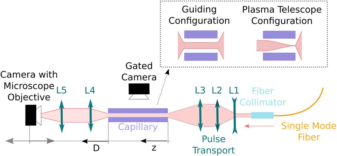
    Figure 1.Schematic overview of the experimental setup. The pulse propagates from right to left. The distance along the capillary is and downstream the capillary is . Optical lenses have the following focal lengths: L, –10 cm; L, 40 cm; L, 150 cm; L, 100 cm; L, 60 cm.

    Applications require reproducible waveguide parameters. For example, the reproducibility of particle bunches accelerated in laser-driven plasma wakefield accelerators (LPAs) is defined by the reproducibility of the wakefield, which is a product of all parts that are involved. Acceleration of high-quality bunches requires every component to be well controlled and stable, i.e., the plasma and the drive bunch or pulse. In this paper, we characterize the plasma to understand the sources of variations. We show that the matched spot size ${w}_m$ was stable and reproducible to $0.05$% for the 9 cm long, to $0.1$% for the 20 cm long, and to $0.2$% for the 40 cm long waveguides. Variations of the longitudinally averaged on-axis plasma electron density were measured to be less than 1%. These results imply that variations caused by a discharge plasma waveguide account for only a small fraction of the parameter variations observed in electron bunches.

    2 Experimental setup

    Figure 1 provides a schematic overview of the experimental setup. We used a laser probe pulse to characterize the plasma channel properties. The pulse was produced by the front end of the BErkeley Lab Laser Accelerator (BELLA) petawatt laser system[27]. Light leaking through a mirror downstream the regenerative amplifier was transported to the experimental area by a single mode optical fiber (see Figure 1). After transport, the pulse had a central wavelength of ${\lambda}_l=780\ \mathrm{nm}$, a pulse length of $\tau \simeq 600$ ps and a focal point spot size adjustable from $\sim 70$ to $105\;\mathrm{\mu} \mathrm{m}$. The pulse energy was $<$4 nJ which is low enough to not modify the channel profile. The capillary was discharged and measurements were obtained at a repetition rate of 1 Hz. The pulse was set to arrive $\sim 0$ to 400 ns after the peak of the discharge current pulse.

    The transverse, time-integrated laser pulse profile was imaged with a charged-coupled-device (CCD) camera, as shown in Figure 1. The camera had 1626 × 1236 pixels and a resolution of 0.935 $\mathrm{\mu} \mathrm{m}$/pixel. The camera was mounted onto a translation stage; the optical setup allowed changing the imaging location from $\sim 30$ cm upstream the capillary entrance to $\sim 40$ cm downstream the capillary exit. Figure 2 (left) shows an example of a measured (single-shot, background subtracted) transverse laser pulse intensity distribution at the focal point location (which was also the location of the capillary entrance aperture).

    Examples of experimentally measured transverse pulse intensity distributions: left, at vacuum focus; center, at the capillary exit plane when the pulse propagated in the 40 cm long capillary #4; right, at the capillary exit plane when the pulse propagated in vacuum. Blue lines show the horizontal and vertical projections of the camera images. Red dotted lines show the results of Gaussian fits of the projections. The left and middle plots are on the same linear color scale; the color scale of the right plot is enhanced by a factor of 10.

    Figure 2.Examples of experimentally measured transverse pulse intensity distributions: left, at vacuum focus; center, at the capillary exit plane when the pulse propagated in the 40 cm long capillary #4; right, at the capillary exit plane when the pulse propagated in vacuum. Blue lines show the horizontal and vertical projections of the camera images. Red dotted lines show the results of Gaussian fits of the projections. The left and middle plots are on the same linear color scale; the color scale of the right plot is enhanced by a factor of 10.

    The plasma was created by a discharge current in a gas-filled capillary. The capillary bulk material was either sapphire $\left({\mathrm{Al}}_2{\mathrm{O}}_3\right)$ or a machinable glass ceramic (MGC). Sapphire is transparent and allows for transverse plasma light diagnostics[28]; the MGC is opaque but is cheaper, can be made longer in a single piece and is easily mechanically machinable. Two gas inlets (located 6 mm from the upstream and downstream capillary ends) allowed filling the capillaries with hydrogen gas. Both capillary ends were open such that gas escapes to the vacuum chamber. Table 1 lists the capillaries that were used for this paper. We chose parameters that are either relevant for laser-driven plasma wakefield acceleration (#1, #2, #4) or plasma telescopes (#3).

    CapillaryMaterialDiameter $\left(\mathrm{\mu} \mathrm{m}\right)$Length (cm)${n}_{i0}$ (atoms/cm${}^3$)${w}_m$ ($\mathrm{\mu} \mathrm{m})$
    #1Sapphire650 $\pm$ 309(1.6–13)$\times$10${}^{17}$105–75
    #2Sapphire830 $\pm$ 5020(0.7–6.6)$\times$10${}^{17}$180–115
    #3MGC2000 $\pm$ 2020(0.65–2.4)$\times$10${}^{17}$$\sim$650–235
    #4MGC830 $\pm$ 2040(1.5–6.6)$\times$10${}^{17}$180–115

    Table 1. Overview of capillary parameters and operation range.

    Electrodes were located at each end of the capillary. Switching capacitors charged to $\sim 20$ kV induced a gas breakdown. The current pulse profile was close to sinusoidal with a rise time between 340 and 420 ns and a peak amplitude between 520 and 620 A (depending on the capillary length and radius, and initial neutral gas pressure). We note that plasma channel properties are only weakly dependent on discharge current pulse length and peak current[22]. The values for the on-axis plasma electron densities ${n}_e(0)$ are known from measurements of the initial neutral gas density that were compared to previous plasma electron densities[29] and range from 0.1$\times {10}^{17}$ to 50$\times {10}^{17}$ electrons/cm${}^3$. The maximum available pressure was limited by the speed of the vacuum pumping system and the lowest available pressure was limited by the timing reproducibility of the discharge. For the sapphire capillaries, spectrally resolved plasma light images suggest that ablation from the capillary walls is negligible for the parameters in Table 1. Aluminum and oxygen spectral lines were observed for lower initial neutral gas densities than in Table 1, where the plasma temperature is higher[30].

    As summarized in Table 1, plasma waveguides of length 9–40 cm were analyzed. Producing shorter channels is typically straightforward. To the best of the authors’ knowledge, 40 cm is the longest discharge capillary waveguide that has been demonstrated. In the context of laser-driven plasma wakefield acceleration, reaching 10 GeV electron energy gain in a single stage requires an on-axis plasma electron density lower than ${n}_e(0)=$2.8$\times {10}^{17}$ electrons/cm${}^3$, based on one-dimensional estimates[23]. At ${n}_e(0)=$2.8$\times {10}^{17}$ electrons/cm${}^3$ the dephasing length is ${L}_d\sim$40 cm for an 800 nm driver. Even longer channels are possible, but may require timing jitter mitigation techniques[3134].

    Capillary #3 has a diameter of 2000 $\mathrm{\mu} \mathrm{m}$, which is more than double of what is typically used for guiding. We tested this capillary to demonstrate the ‘plasma telescope’ concept (see Figure 1), a compact way to modify laser pulse spot size. Large diameter capillaries are also interesting for particle bunch transport, where the capillary radius often limits particle acceptance or the maximum bunch size. Larger bunch sizes (and, therefore, lower bunch intensities) are desired to minimize wakefield effects in active plasma lenses. Even larger diameters are possible, but require an increase in the speed of the vacuum pumping system.

    3 Experimental results

    3.1 Measurement of the matched spot size

    Figure 2 shows examples of transverse pulse intensity distributions measured when using the 40 cm long capillary #4: the left image shows the pulse at the capillary entrance (which is also the location of the focal point); the right image shows the central section of the pulse after 40 cm of vacuum propagation (root-mean-square (rms) spot size $\sim 300$$\ \mathrm{\mu} \mathrm{m}$); the center image shows an example of the pulse in the capillary exit plane after transport in the plasma waveguide. The transverse intensity distribution of the guided pulse was similar to the input pulse.

    We estimated the waveguide energy transmission ${E}_t$ by comparing the total counts of the background subtracted pulse input and output camera images. Within the error of this measurement ($\Delta {E}_t\sim$ 2%) and for reasonable experimental settings, the energy transmission was approximately 100%. All energy that enters the waveguide exits. Thus, pulse scattering off the plasma is negligible for waveguides with a density-length product of up to at least 6$\times {10}^{18}$ (atoms/cm${}^3)\times$cm.

    Plasma channels focus laser pulses due to a radially varying refractive index. The profile is defined by the radial plasma electron density distribution $\Delta {n}_e(r)$, which is defined by thermal effects and is closely tied to the capillary radius. The smaller the radius, the steeper the temperature gradient, the stronger the focusing strength of the channel. The matched spot size ${w}_m$ can be obtained from the radial electron density distribution according to[35]

    $$\begin{align}8\pi {r}_e{\int}_0^{\infty}\left[{n}_e(r)\left(\frac{2{r}^2}{w_m^2}-1\right){e}^{-\frac{2{r}^2}{w_m^2}}\right]r\; \mathrm{d}r-1=0,\end{align}$$ 

    where $r$ is the radial coordinate. The spot size evolution of a transversely Gaussian, low-intensity pulse that is focused at the entrance of a parabolic channel is described by[24]

    $$\begin{align}{w}^2(z)=\frac{w_i^2}{2}\left[1+\frac{w_m^4}{w_i^4}+\left(1-\frac{w_m^4}{w_i^4}\right)\cos \left(\frac{2\pi z}{\lambda_{\mathrm{osc}}}\right)\right],\end{align}$$ 

    where $w$ is the transverse spot size at the location $z$ along the waveguide, ${w}_i$ is the input spot size and ${\lambda}_{\mathrm{osc}}$ is the spot size oscillation length. Unless the pulse propagation axis overlaps with the channel axis, the pulse centroid position oscillates along the channel. The pulse centroid position at the capillary exit ${O}_{\mathrm{pulse}}$ (with respect to the incoming laser axis) is defined by the trajectory of the pulse centroid along the channel. When the transverse channel profile is parabolic and the incident low-power pulse parallel to the waveguide axis, the centroid oscillations can be described by[24]

    $$\begin{align}{x}_c={x}_i\kern0.1em \cos \left(\frac{4\pi z}{\lambda_{\mathrm{osc}}}\right),\end{align}$$ 

    where ${x}_i$ is the offset between the pulse propagation and waveguide axis.

    Measuring the pulse centroid position at the capillary exit ${O}_{\mathrm{pulse}}$ as a function of the offset between the pulse and capillary axis ${O}_{\mathrm{cap}}$ (defined by the translation of the capillary axis with respect to the incoming laser axis) allows for evaluation of the matched spot size of a parabolic channel. The technique is described in Ref. [24]. If the channel is parabolic, the measured relation is linear and the matched spot size can be calculated from

    $$\begin{align}{w}_m=\sqrt{\frac{2z}{k\left[{\mathrm{arccos}}\left(\mathrm{d}{O}_{\mathrm{pulse}}/\mathrm{d}{O}_{\mathrm{cap}}\right)+2\pi j\right]}},\end{align}$$ 

    where ${\mathrm{d}O}_{\mathrm{pulse}}/{\mathrm{d}O}_{\mathrm{cap}}$ is the near-axis derivative of ${O}_{\mathrm{pulse}}$ versus ${O}_{\mathrm{cap}}$ and $k$ is the laser wavenumber. In this work the integer $j$ was determined by measuring the response of the laser pulse to the initial neutral gas density.

    Figure 3(a) shows the measured relation of ${O}_{\mathrm{pulse}}$ as a function of ${O}_{\mathrm{cap}}$ for capillary #1 and an initial neutral gas density number of ${n}_{i0}=6.5\times {10}^{17}$ atoms/cm${}^3$. The pulse centroid position was defined from Gaussian fits to the projections of the measured pulse intensity distributions. Measurement ranges were limited to $\mid {O}_{\mathrm{cap}}\mid \lesssim 200$$\ \mathrm{\mu} \mathrm{m}$ as for larger values of ${O}_{\mathrm{cap}}$ the pulse interacted with the capillary walls.

    Reconstructed radial plasma electron density profile. (a) Measurements of the centroid position of the guided pulse at the capillary exit as a function of the parallel capillary offset with respect to the laser propagation axis (green markers). Error bars (standard deviation of the individual measurements) are not visible because they are smaller than the marker size. The blue line shows a linear fit to the data; it is solid over the measurement range and dashed outside (assuming the continuation of a parabolic channel outside the measurement range). (b) Calculated relative change of the radial plasma electron density (green markers) compared with one-dimensional NPINCH simulation results (gray line). The blue line corresponds to the result of the fit shown in panel (a).

    Figure 3.Reconstructed radial plasma electron density profile. (a) Measurements of the centroid position of the guided pulse at the capillary exit as a function of the parallel capillary offset with respect to the laser propagation axis (green markers). Error bars (standard deviation of the individual measurements) are not visible because they are smaller than the marker size. The blue line shows a linear fit to the data; it is solid over the measurement range and dashed outside (assuming the continuation of a parabolic channel outside the measurement range). (b) Calculated relative change of the radial plasma electron density (green markers) compared with one-dimensional NPINCH simulation results (gray line). The blue line corresponds to the result of the fit shown in panel (a).

    In Figure 3(a), ${O}_{\mathrm{pulse}}$ was a linear function of ${O}_{\mathrm{cap}}$ over the measurement range. The result is consistent with the pulse experiencing a parabolic channel profile ($\Delta {n}_e(r)$ according to Equation (2)). We then used Equation (6) to calculate ${w}_m$ and show the resulting radial distribution of the plasma electron density in Figure 3(b) (blue line). Measurements yielded excellent agreement with one-dimensional magnetohydrodynamic (MHD) simulations results (gray line). The simulations were performed with the one-dimensional code NPINCH[36], using the experimental capillary and atomic density parameters as input. These simulations are consistent with previous theoretical and simulation work[21] showing that capillary discharge waveguides do not produce parabolic density profiles over the entire capillary transverse extent. However, over a sufficiently small radius ($\mid {O}_{\mathrm{cap}}\mid \gtrsim 200$$\ \mathrm{\mu} \mathrm{m}$), a parabolic assumption is reasonable (see Figure 3(b)).

    We performed horizontal and vertical centroid oscillation measurements for all capillaries over the accessible density range. Values for ${w}_m$ are summarized in Table 1[37]. The matched spot size obtained from horizontal and vertical measurements agreed within 2%. In addition, when the pulse propagation axis was approximately aligned to the waveguide axis, the guided pulse intensity distributions were radially symmetric (for all tested capillaries, see, e.g., Figures 2 and 7(c)) and the horizontal and vertical pulse sizes agreed to better than $<1$$\ \mathrm{\mu} \mathrm{m}$ (or 1.4%) for the 9 cm long, $<3\ \mathrm{\mu} \mathrm{m}$ (or 2.7%) for the 20 cm long, and $<3$$\ \mathrm{\mu} \mathrm{m}$ (or 2.7%) for the 40 cm long waveguides. Therefore, the matched spot size was symmetric to better than 3%.

    3.2 Waveguide parameter reproducibility

    Applications and multi-shot measurements require channel properties to be stable and reproducible from discharge to discharge. Parameters such as the channel central axis, the focusing strength, or the on-axis plasma electron density are demanded to be repeatable from event to event and stable over long timescales. For example, variations in the matched spot size change the pulse evolution inside the waveguide as well as the pulse divergence downstream. To evaluate waveguide parameter variations, we observed their effects on the probe pulse. We also decided to use a combination of capillary length $L$ and matched spot size ${w}_m$ for which:

    1. (i)the transverse spot size at the capillary exit was equal to the pulse vacuum focal spot size; the spot underwent an integer number $n$ of oscillations, $L=n{\lambda}_{\mathrm{osc}}$; analysis of a similar sized input and guided pulse facilitated the interpretation of the results;
    2. (ii)the pulse centroid position underwent approximately half an integer number of oscillations, $L=\left(n/2\right){\lambda}_{\mathrm{osc}}$, such that the pulse centroid offset at the capillary exit plane was maximized and measurement sensitivity optimized.

    We chose capillary #1 (9 cm length[38]) together with an initial neutral gas density of ${n}_{i0}=6.5\times 1{0}^{17}$ atoms/cm${}^3$ that resulted in a matched spot size of ${w}_m=$88.8  $\,\mathrm{\mu} \mathrm{m}$ (see Figure 3). For the 780 nm probe pulse, the theoretical spot size oscillation length was ${\lambda}_{\mathrm{osc}}$=9.9 cm and the centroid oscillation length was $2{\lambda}_{\mathrm{osc}}$=19.8 cm. The pulse therefore underwent approximately half a centroid position oscillation and a full spot size oscillation along the capillary.

    Figure 4(a) compares variations of the guided pulse centroid position at the capillary exit (orange) with those of the incoming pulse at the capillary entrance (blue). The pulse centroid was defined as the location of the peak of the Gaussian fit to the projections. Deviations from the centroid reference $c$ are the quadratic sums of the horizontal ${c}_x$ and vertical ${c}_y$ contributions $\left(c=\sqrt{c_x^2+{c}_y^2}\right)$. The top plot of Figure 4 compares the running average of 100 measured pulse centroid deviations $C=c-\overline{c}$, where the mean centroid position $\overline{c}$ was subtracted from the individual measurement $c$; the bottom plot of Figure 4 compares running average of 100 pulse spot size deviations $W=w-\overline{w}$, where the mean spot size $\overline{w}=\left(74\pm 1\right)$$\ \mathrm{\mu} \mathrm{m}$ was subtracted from the individual measurement $w$. Respectively colored error bands show the running average of the standard deviations of 100 measurements.

    (a) Pulse centroid position variations , where is the measured pulse center and the average value of all measurements; (b) spot size deviations , where is the rms pulse size and the average value of all measurements. The figure shows the running average of 100 measurements (solid line) as well as their standard deviation (error-band) for capillary #1. Measurements for the incoming pulse at the capillary entrance are shown in blue and those for the guided pulse at the capillary exit in orange. (c) Correlation between and the timing jitter between the discharge and the probe pulse () for an initial neutral gas density of atoms/cm for capillary #2. The green dashed line shows the result of a linear fit.

    Figure 4.(a) Pulse centroid position variations , where is the measured pulse center and the average value of all measurements; (b) spot size deviations , where is the rms pulse size and the average value of all measurements. The figure shows the running average of 100 measurements (solid line) as well as their standard deviation (error-band) for capillary #1. Measurements for the incoming pulse at the capillary entrance are shown in blue and those for the guided pulse at the capillary exit in orange. (c) Correlation between and the timing jitter between the discharge and the probe pulse () for an initial neutral gas density of atoms/cm for capillary #2. The green dashed line shows the result of a linear fit.

    From the data presented in Figure 4(a) we calculated the standard deviation of all measurements. Variations of the incoming pulse $\Delta C$ = 2.7 $\mathrm{\mu} \mathrm{m}$ are rms and were equal to those of the guided pulse. This means that within the resolution of the measurement ($1$$\ \mathrm{\mu} \mathrm{m}$), the central position of the created plasma channel was repeatable and stable over the measured timescale. The overall length of the measurements was limited to $\sim$30 minutes by a thermal drift of the incoming probe pulse, which could be mitigated in the future with active pointing feedback.

    The rms spot size variation $\Delta W$ (Figure 4(b)) increased after guiding by $\Delta W$ = 0.04 $\mathrm{\mu} \mathrm{m}$ (see the bottom plot of Figure 4). Spot-size variations are a result of the variations of the matched spot size. The measured values translate to variations of ${w}_m$ around 0.05%. This increase in $\Delta W$ was measurable, but negligible with respect to the absolute spot size of $\overline{w}$=74 $\mathrm{\mu} \mathrm{m}$ and translates to pulse peak intensity variations $\Delta I$ of $\sim$0.1% for ${w}_0={w}_m$.

    We performed the same set of measurements for capillaries #2 and #4. There was no measurable increase in $\Delta C$. Spot size variations increased by $\Delta W$ = 0.26 $\mathrm{\mu} \mathrm{m}$ for capillary #2 and $\Delta W$ = 0.52 $\mathrm{\mu} \mathrm{m}$ for capillary #4, corresponding to 0.5% and 1% in pulse peak intensity variations (when ${w}_0={w}_m$). They translate to variations in matched spot size that are around 0.1% for capillary #2 and 0.2% for capillary #4.

    We found that for capillaries longer than 20 cm, part of the increase in spot size variations could be explained by timing jitter between the discharge and the laser pulse arrival time ($\Delta t$). Experiments showed that the amplitude of the timing jitter depends on the initial neutral gas density (${n}_{i0}$), the capillary length and radius as well as the discharge voltage. For example, for ${n}_{i0}=2\times {10}^{17}$ atoms/cm${}^3$ the rms value of the timing jitter was $\Delta t\sim$ 5 ns for the 20 cm long capillary #2, $\Delta t=$12 ns for the 2 mm diameter capillary #3, and $\Delta t=$9 ns for the 40 cm long capillary #4. Figure 4(c) shows the correlation measurement for capillary #2 for ${n}_{i0}=2\times {10}^{17}$ atoms/cm${}^3$ as well as the result of a linear fit to the measurements (green dashed line). Improving the discharge timing jitter[31] by, e.g., using an additional current pulse[32] to create the plasma, operating at a higher discharge voltage or using a laser trigger[33,34] could decrease variations by, e.g., $\Delta W$ = 0.11 $\mathrm{\mu} \mathrm{m}$ (or –20%) in the case of capillary #2. The correlation was not measurable with capillary #1 as jitter values were below $\Delta t<$1 ns.

    For our laser pulse input parameters and the minimum matched spot size of capillary #3 $\left({w}_m>230\;\mathrm{\mu} \mathrm{m}\right)$ the pulse at the capillary exit was always much larger than the input and showed significant higher-order mode contributions (see Section 4.2). This resulted in limited accuracy in the measurement of the centroid (see condition (ii)) and spot size variations and results are therefore not presented. In the future the laser angle exiting from the waveguide could be measured to increase accuracy.

    3.3 Observation of higher order contributions to the transverse channel profile

    The excellent reproducibility of the waveguide is a prerequisite for applications, e.g., to produce stable electron bunches from an LPA. Together with a reproducible probe pulse it also enabled measurements of the transverse channel profile with unprecedented precision. Figure 5(b) shows a centroid oscillation measurement for the 2000 $\mathrm{\mu} \mathrm{m}$ diameter capillary #3 (green dots). The alignment offset was limited to $\mid {O}_{\mathrm{cap}}\mid \lesssim 700$$\ \mathrm{\mu} \mathrm{m}$; outside this range the laser pulse interacted with the capillary walls and accurate identification of the pulse centroid position was no longer possible. For $\mid {O}_{\mathrm{cap}}\mid \gtrsim 500$$\ \mathrm{\mu} \mathrm{m}$, the guided pulse intensity distribution deviated from Gaussian; the pulse centroid position was therefore calculated from the center of mass.

    Reconstructed radial plasma electron density profile. (a) Measurements of the centroid position of the guided pulse at the capillary exit (green markers) as a function of the parallel capillary offset with respect to the laser propagation axis . Error bars (standard deviation of the individual measurements) are not visible as they are smaller than the marker size. The blue and red solid (within the measurement range) and dashed (outside the measurement range) lines show the calculated centroid oscillation scan result corresponding to the density profiles of the same color on the right. (b) Calculated relative change of the plasma electron density as a function of radial position for a parabolic channel (blue line), a channel with an component (red line) compared with the result from NPINCH simulations (gray line).

    Figure 5.Reconstructed radial plasma electron density profile. (a) Measurements of the centroid position of the guided pulse at the capillary exit (green markers) as a function of the parallel capillary offset with respect to the laser propagation axis . Error bars (standard deviation of the individual measurements) are not visible as they are smaller than the marker size. The blue and red solid (within the measurement range) and dashed (outside the measurement range) lines show the calculated centroid oscillation scan result corresponding to the density profiles of the same color on the right. (b) Calculated relative change of the plasma electron density as a function of radial position for a parabolic channel (blue line), a channel with an component (red line) compared with the result from NPINCH simulations (gray line).

    The blue line in Figure 5(a) shows a linear fit (according to Equation (6)) to the centroid oscillation result. It does not provide a good description of the measurement for $\mid {O}_{\mathrm{cap}}\mid >400$$\ \mathrm{\mu} \mathrm{m}$. To find a model that can describe the results better, we calculated the centroid position response to different radial electron density distributions ${n}_e(r)$. We found that the following equation provides an excellent description of the measurements in general, as was predicted in Ref. [35]:

    $$\begin{align}{n}_e(r)={n}_e(0)+\frac{1-{E}_{\psi}}{\pi {r}_e{w}_m^4}{r}^2+\frac{E_{\psi }}{2\pi {r}_e{w}_m^6}{r}^4,\end{align}$$ 

    where ${E}_{\psi }$ is a scaling factor for the relative contributions of the ${r}^2$ and ${r}^4$ terms. When ${E}_{\psi }=0$, the radial channel profile is parabolic, equal to Equation (2).

    Figure 5(a) shows that adding an ${r}^4$ (${E}_{\psi }>0$) component to the radial plasma electron density profile (red line) according to Equation (7) allowed to greatly improve the agreement between the model (${E}_{\psi }$ and ${w}_m$ are free parameters) and the measurement. We calculated the result of centroid oscillation scans for different parameters of ${w}_m$ and ${E}_{\psi }$ until the average deviation between measurements and the model was minimized. Figure 5(a) shows the relative radial plasma electron densities that correspond to the models shown in Figure 5(b). A comparison with NPINCH simulation results (gray line) confirmed that the channel profile rises stronger than the parabolic (blue line, ${E}_{\psi }=0$). Simulation results also indicate that a description of the channel profile close to the capillary walls ($\mid r\mid \gtrsim 700$$\ \mathrm{\mu} \mathrm{m}$, outside the measured range) may require adding additional higher-order terms to Equation (7).

    Figures 3(b) and 5(b) show that the central regions ($\mid r\mid \lesssim 2{w}_m$) of the measured channel profiles were well described by Equation (2). For $\mid r\mid >2{w}_m$, the ${r}^4$ contribution became significant, with increasing values of ${E}_{\psi }$ for larger capillary diameters and higher initial neutral gas pressures. Values of ${E}_{\psi }$ varied only slightly with discharge timing and initial neutral gas density. Over our measurement range (see Table 1) they range from $0.05<{E}_{\psi }<0.15$ for capillaries #2 and #4, and from $0.1<{E}_{\psi }<0.2$ for capillary #3. For capillary #1 they were generally small (below ${E}_{\psi }<0.05$). Outside the measurement ranges (see red and blue dashed lines in Figure 3(b) and 5(b)), there is a discrepancy between the models and the NPINCH simulation result. Polynomial fits to NPINCH simulation results revealed that all capillary diameters require an additional ${r}^6$ term to obtain a good description of the density profile close to the capillary walls.

    Waterfall plot of the simulated pulse intensity evolution downstream the capillary exit . The red dashed line shows the rms spot size from Gaussian fits to the intensity distribution from the simulations for a parabolic channel using (red). The green line shows the measured evolution of the rms size of the pulse after guiding. The blue line shows the pulse evolution downstream the vacuum focus.

    Figure 6.Waterfall plot of the simulated pulse intensity evolution downstream the capillary exit . The red dashed line shows the rms spot size from Gaussian fits to the intensity distribution from the simulations for a parabolic channel using   (red). The green line shows the measured evolution of the rms size of the pulse after guiding. The blue line shows the pulse evolution downstream the vacuum focus.

    (a) Simulation result of the laser pulse intensity evolution along the capillary #3 in a plasma telescope configuration, using the channel profile according to Figure 5 as input. (b) Simulated pulse intensity evolution downstream the capillary exit . Orange markers show the second moment of the pulse obtained from experimental measurements. The gray vertical dashed line indicates the location of the measured intensity distributions shown in (c)–(f). (c) The experimentally measured intensity profile, (d) the corresponding simulation result when using the Gerchberg–Sexton algorithm to reconstruct the input pulse modes, (e) when using a perfect Gaussian pulse as simulation input, and (f) when using a Gaussian pulse that was matched to the channel with .

    Figure 7.(a) Simulation result of the laser pulse intensity evolution along the capillary #3 in a plasma telescope configuration, using the channel profile according to Figure 5 as input. (b) Simulated pulse intensity evolution downstream the capillary exit . Orange markers show the second moment of the pulse obtained from experimental measurements. The gray vertical dashed line indicates the location of the measured intensity distributions shown in (c)–(f). (c) The experimentally measured intensity profile, (d) the corresponding simulation result when using the Gerchberg–Sexton algorithm to reconstruct the input pulse modes, (e) when using a perfect Gaussian pulse as simulation input, and (f) when using a Gaussian pulse that was matched to the channel with   .

    4 Implications of parameter reproducibility and non-parabolic channel contributions for applications

    4.1 LPAs

    When using waveguides in the context of laser-driven plasma wakefield acceleration the matched spot size ${w}_m$ is typically chosen to be close to the pulse focal spot size ${w}_0$. The pulse is contained to the parabolic region ($w\sim {w}_m$) of the channel. For these circumstances, as shown in Figure 6, we experimentally observed that the pulse evolution downstream the capillary exit (green solid line) was approximately equal to the pulse evolution downstream vacuum focus (blue solid line). There is good agreement between the two measurements, over approximately two Rayleigh ranges $\left({Z}_r\sim 2.2\; \mathrm{cm}\right)$, which shows that pulse quality was not degraded.

    To confirm that the radial profile measured in Section 3.1 is consistent with the evolution of the pulse exiting from the waveguide, propagation simulations were performed. The pulse mode was retrieved from a Gerchberg–Sexton algorithm on the measured fluence evolution along the propagation axis $z$. We performed INF&RNO[39,40] calculations using this mode as input. The plasma channel was modeled according to the results of Figure 3, parabolic with ${{w}_m=88.8\ \mathrm{\mu} \mathrm{m}}$. Along the plasma, the density profile was uniform with linear density ramps to vacuum at each end. Figure 6 shows the simulated pulse intensity evolution downstream the capillary exit $\left(D=0\right).$ On top of the waterfall plot of the pulse intensity, we compare the results of Gaussian fits on the simulated (red dashed line) and measured (green solid line) data. The good agreement between the two curves confirmed the experimentally measured channel profile from Figure 3.

    In Section 3.2 we demonstrated the excellent reproducibility of the waveguide parameters that control pulse guiding (second term on the right-hand side of Equation (2)). For capillary #2, the matched spot size was repeatable to 0.1%. Changing the matched spot size by $\sim$0.1%, for example from 88.8 $\mathrm{\mu} \mathrm{m}$ to 88.9 $\mathrm{\mu} \mathrm{m}$, changes the pulse peak intensity of a Gaussian pulse with a spot size of ${w}_0=$88.8 $\mathrm{\mu} \mathrm{m}$ by 0.25%. These variations translate to a change in the laser strength parameter ${a}_0$ of 0.12%. The pulse peak intensity variations caused by the waveguide are therefore much smaller than typical intensity variations ($\sim 10$%) at the focal plane of petawatt class laser systems[27].

    LPAs additionally require reproducibility of the on-axis plasma electron density ${n}_e(0)$ (first term on the right-hand side of Equation (2)): plasma electron density variations result, e.g., in variations of the accelerating gradient as the wakefield phase and amplitude change. We evaluated variations of ${n}_e(0)$ by using a group velocity dispersion (GVD) technique described in Ref. [29]. Longitudinal average plasma density values are obtained by tracking the phase of interference fringes. Measurements were performed on capillary #2 on the BELLA petawatt experimental setup[27,41] for an on-axis density of ${n}_e=2\times 1{0}^{17}$ electrons/cm${}^3$ and were $<$1% (with accuracy limited by probe pulse fluctuations). At ${n}_e=2\times 1{0}^{17}$ electrons/cm${}^3$ the peak accelerating field (estimated based on the cold plasma wave-breaking limit) is 43 GV/m. A 1% variation in ${n}_e(0)$ translates to changes of $\sim$0.22 GV/m or $\sim$0.5%, much smaller than the variations that are typically observed in experiments[42,43].

    The two major components of LPAs are the laser and the plasma. Our measurement results highlight that discharge plasma waveguide parameter variations are small compared with typical variations of the pulses produced by LPA laser systems. Thus, increased laser pulse parameter reproducibility is essential to achieve significant improvements in the reproducibility and stability of particle bunches, consistent with the findings of Ref. [44].

    4.2 Plasma telescopes

    Waveguides could also be used as ‘plasma telescopes’: for the right combination of capillary length and matched spot size the pulse exits from the plasma after half a spot-size oscillation, changing it from ${w}_0$ to ${w}_m^2/{w}_0$. This feature may be used to increase or decrease the spot size of a high-intensity pulse in a short distance, where conventional optics would be destroyed.

    To understand how the ${r}^4$ component in Equation (7) affects pulse propagation for waveguides that are used as plasma telescopes, we performed measurements on the 2 mm diameter capillary #3. We placed the capillary entrance 20 cm downstream the pulse focus (${w}_0\sim$105 $\mathrm{\mu}$m) and used the waveguide (see Figure 5) to ‘collimate’ the diverging pulse. Measurements of the pulse profile downstream the waveguide showed that the pulse is no longer transversely Gaussian (see Figure 7(c)). A radially symmetric ring structure was clearly visible. The pulse spot size (calculated from the second moment of the transverse intensity distribution) oscillated downstream the waveguide as shown by orange points in Figure 7(b).

    We simulated pulse propagation with INF&RNO, using the reconstructed input pulse and the NPINCH channel profile from Figure 5. Figure 7(a) shows the pulse evolution inside the capillary and Figure 7(b) downstream the capillary exit. The transverse pulse intensity distribution downstream the capillary exit showed higher-order modes, qualitatively similar to the experimental measurements; the pulse peak intensity as well as its spot size oscillated as different modes came in and out of focus. Figures 7(c)–7(e) compare transverse pulse intensity distributions 20 cm downstream the capillary exit. Figure 7(c) is the experimentally measured distribution; Figure 7(d) was obtained from simulations when using a model of the input pulse; and Figure 7(e) from simulations when using a transversely Gaussian input pulse. Figures 7(c)–7(e) all show the same ‘ring’ features, even when the input pulse is a perfect Gaussian (Figure 7(e)); the ‘ring’ features are therefore a result of the pulse experiencing the non-parabolic contributions of Equation (7). These initial experiments highlighted that research and development will be required before capillary discharge waveguides can be used as plasma telescopes for applications that require a Gaussian mode.

    Figure 7(f) shows the simulated transverse pulse intensity distribution 20 cm downstream the capillary exit for a pulse (${w}_0=245$$\ \mathrm{\mu}$m) that was matched to the plasma channel (${w}_m=245$$\ \mathrm{\mu} \mathrm{m}$, ${E}_{\psi }=0.12$). Non-Gaussian features were negligible. This simulation result confirms that when ${w}_0\sim {w}_m$, the effects of non-parabolic channel contributions on pulse propagation are insignificant.

    5 Conclusions and summary

    We evaluated the reproducibility of plasma channels formed by discharges in gas-filled capillary waveguides and obtained precise measurements of their radial plasma electron density distributions. Variations of the waveguide central axis were below the 1 $\mathrm{\mu} \mathrm{m}$ resolution of the measurement; variations of the average on-axis density had an upper limit of 1%. Matched spot size variations were largest ($\Delta {w}_m=$0.2%) for the longest capillary (40 cm). We project that these quantities are not sufficient to cause the large electron beam parameter variations that are typically observed in laser-driven plasma wakefield acceleration experiments to date[42,43]. Improvements of the quality and reproducibility of particle bunches accelerated in laser-driven plasma wakefields therefore require improvements of the laser pulse parameter variations[44].

    Measurements of the transverse waveguide profiles revealed non-parabolic contributions to the radial channel profile that were in excellent agreement with MHD simulation results. We have demonstrated that non-parabolic effects influenced pulse propagation for non-matched waveguide applications, such as plasma telescopes. However, when the pulse was approximately matched to the waveguide, their effects were negligible.

    References

    [1] D. J. Spence, A. Butler, S. M. Hooker. J. Opt. Soc. Am. B, 20, 138(2003).

    [2] T. Higashiguchi, M. Hikida, H. Terauchi, J. Bai, T. Kikuchi, Y. Tao, N. Yugami. Rev. Sci. Instrum., 81, 046109(2010).

    [3] C. G. Durfee, H. M. Milchberg. Phys. Rev. Lett., 71, 2409(1993).

    [4] J. J. Su, T. Katsouleas, J. M. Dawson, R. Fedele. Phys. Rev. A, 41, 3321(1990).

    [5] J. van Tilborg, S. Steinke, C. G. R. Geddes, N. H. Matlis, B. H. Shaw, A. J. Gonsalves, J. V. Huijts, K. Nakamura, J. Daniels, C. B. Schroeder, C. Benedetti, E. Esarey, S. S. Bulanov, N. A. Bobrova, P. V. Sasorov, W. P. Leemans. Phys. Rev. Lett., 115, 184802(2015).

    [6] E. Brentegani, P. Anania, S. Atzeni, A. Biagioni, E. Chiadroni, M. Croia, M. Ferrario, F. Filippi, A. Marocchino, A. Mostaccia, R. Pompili, S. Romeo, A. Schiavi, A. Zigler. Nucl. Instrum. Methods Phys. Res. A, 909, 404(2018).

    [7] E. Chiadroni, M. P. Anania, M. Bellaveglia, A. Biagioni, F. Bisesto, E. Brentegani, F. Cardelli, A. Cianchi, G. Costa, D. Di Giovenale, G. Di Pirro, M. Ferrario, F. Filippi, A. Gallo, A. Giribono, A. Marocchino, A. Mostacci, L. Piersanti, R. Pompili, J. B. Rosenzweig, A. R. Rossi, J. Scifo, V. Shpakov, C. Vaccarezza, F. Villa, A. Zigler. Nucl. Instrum. Methods Phys. Res. A, 909, 16(2018).

    [8] P. Sprangle, E. Esarey, J. Krall, G. Joyce. Phys. Rev. Lett., 69, 2200(1992).

    [9] J. van Tilborg, S. K. Barber, C. Benedetti, C. B. Schroeder, F. Isono, H.-E. Tsai, C. G. R. Geddes, W. P. Leemans. Phys. Plasmas, 25, 056702(2018).

    [10] C. G. R. Geddes, C. Toth, J. van Tilborg, E. Esarey, C. B. Schroeder, J. Cary, W. P. Leemans. Phys. Rev. Lett., 95, 145002(2005).

    [11] R. Pompili, M. P. Anania, E. Chiadroni, A. Cianchi, M. Ferrario, V. Lollo, A. Notargiacomo, L. Picardi, C. Ronsivalle, J. B. Rosenzweig, V. Shpakov, A. Vannozzi. Rev. Sci. Instrum., 89, 033302(2018).

    [12] Z. Qin, W. Li, J. Liu, J. Liu, C. Yu, W. Wang, R. Qi, Z. Zhang, M. Fang, K. Feng, Y. Wu, L. Ke, Y. Chen, C. Wang, R. Li, Z. Xu. Phys. Plasmas, 25, 043117(2018).

    [13] S. Karsch, J. Osterhoff, A. Popp, T. P. Rowlands-Rees, Z. Major, M. Fuchs, B. Marx, R. Hoerlein, K. Schmid, L. Veisz, S. Becker, U. Schramm, B. Hidding, G. Pretzler, D. Habs, F. Gruener, F. Kraus, S. M. Hooker. New J. Phys., 9, 415(2007).

    [14] P. Sprangle, E. Esarey, A. Ting, G. Joyce. Appl. Phys. Lett., 53, 2146(1988).

    [15] P. A. Franken, A. E. Hill, C. W. Peters, G. Weinreich. Phys. Rev. Lett., 7, 118(1961).

    [16] D. M. Gaudiosi, B. Reagan, T. Popmintchev, M. Grisham, M. Berrill, O. Cohen, B. C. Walker, M. M. Murnane, H. C. Kapteyn, J. J. Rocca. Phys. Rev. Lett., 96, 203001(2006).

    [17] M. Grisham, D. M. Gaudiosi, B. Reagan, T. Popmintchev, M. Berrill, O. Cohen, B. C. Walker, M. M. Murnane, H. C. Kapteyn, J. J. Rocca. X-Ray Lasers 2006, 383.

    [18] S. Sakai, T. Higashiguchi, N. Bobrova, P. Sasorov, J. Miyazawa, N. Yugami, Y. Sentoku, R. Kodama. Rev. Sci. Instrum., 82, 103509(2011).

    [19] A. Butler, A. J. Gonsalves, C. M. McKenna, D. J. Spence, S. M. Hooker, S. Sebban, T. Mocek, I. Bettaibi, B. Cros. Phys. Rev. Lett., 91, 205001(2003).

    [20] T. Mocek, C. M. McKenna, B. Cros, S. Sebban, D. J. Spence, G. Maynard, I. Bettaibi, V. Vorontsov, A. J. Gonsavles, S. M. Hooker. Phys. Rev. A, 71, 013804(2005).

    [21] N. Bobrova, A. A. Esaulov, J.-I. Sakai, P. V. Sasorov, D. J. Spence, A. Butler, S. M. Hooker, S. V. Bulanov. Phys. Rev. E, 65, 016407(2001).

    [22] B. H. P. Broks, K. Garloff, J. J. A. M. van der Mullen. Phys. Rev. E, 71, 016401(2005).

    [23] E. Esarey, C. B. Schroeder, W. P. Leemans. Rev. Mod. Phys., 81, 1229(2009).

    [24] A. J. Gonsalves, K. Nakamura, C. Lin, J. Osterhoff, S. Shiraishi, C. B. Schroeder, C. G. R. Geddes, Cs. Tóth, E. Esarey, W. P. Leemans. Phys. Plasmas, 17, 056706(2010).

    [25] A. J. Gonsalves, T. P. Rowlands-Rees, B. H. P. Broks, J. A. M. van der Mullen, S. M. Hooker. Phys. Rev. Lett., 98, 025002(2007).

    [26] B. H. P. Broks, W. Van Dijk, J. J. A. W. van der Mullen. Phys. Plasmas, 14, 023501(2007).

    [27] K. Nakamura, H. Mao, A. J. Gonsalves, H. Vincenti, D. E. Mittelberger, J. Daniels, A. Magana, C. Toth, W. P. Leemans. IEEE J. Quantum Electron., 53, 1200121(2017).

    [28] We monitor longitudinal uniformity by imaging the light emitted by the discharge onto the gated camera shown in Figure 1 (gate time 3 ns)..

    [29] C. V. Pieronek, A. J. Gonsalves, C. Benedetti, S. S. Bulanov, J. van Tilborg, J. H. Bin, K. K. Swanson, J. Daniels, G. A. Bagdasarov, N. A. Bobrova, V. A. Gasilov, G. Korn, P. V. Sasorov, C. G. R. Geddes, C. B. Schroeder, W. P. Leemans, E. Esarey. Phys. Plasmas, 27, 093101(2020).

    [30] A. J. Gonsalves, C. Pieronek, J. Daniels, S. S. Bulanov, W. L. Waldron, D. E. Mittelberger, W. P. Leemans, N. A. Bobrova, P. V. Sasorov, F. Liu, S. Antipov, J. E. Butler. J. Appl. Phys., 119, 033302(2016).

    [31] D. Huang, L. J. Yang, P. Huo, J. B. Ma, W. D. Ding, W. Wang. Phys. Plasmas, 22, 023509(2015).

    [32] D. Kaganovich, P. V. Sasorov, Y. Ehrlich, C. Cohen, A. Zigler. Appl. Phys. Lett., 71, 2925(1997).

    [33] C. J. Woolley, K. O’Keeffe, H. K. Chung, S. M. Hooker. Plasma Sources Sci. Technol., 20, 055014(2011).

    [34] B. Greenberg, M. Levin, A. Pukhov, A. Zigler. Appl. Phys. Lett., 83, 2961(2003).

    [35] C. Benedetti, C. B. Schroeder, E. Esarey, W. P. Leemans. Phys. Plasmas, 19, 053101(2012).

    [36] N. A. Boborova, S. V. Bulanov, T. L. Razinkova, P. V. Sasorov. Plasma. Phys. Rep., 22, 349(1996).

    [37] The obtained values vary only by a small amount as a function of discharge timing as long as the pulse arrives in the range of 0–400 ns after the peak of the discharge..

    [38] W. P. Leemans, A. J. Gonsalves, H.-S. Mao, K. Nakamura, C. Benedetti, C. B. Schroeder, C. Tóth, J. Daniels, D. E. Mittelberger, S. S. Bulanov, J.-L. Vay, C. G. R. Geddes, E. Esarey. Phys. Rev. Lett., 113, 245002(2014).

    [39] C. Benedetti, C. Schroeder, E. Esarey, C. Geddes, W. Leemans. AIP Conf. Proc., 1299(2010).

    [40] C. Benedetti, C. Schroeder, C. Geddes, E. Esarey, W. Leemans. Plasma Phys. Control. Fusion, 60(2017).

    [41] W. P. Leemans, A. J. Gonsalves, K. Nakamura, H.-S. Mao, C. Toth, J. Daniels, D. Mittelberger, C. Benedetti, S. Bulanov, C. G. R. Geddes, J.-L. Vay, C. B. Schroeder, E. H. EsareyCLEO: Applications and Technology. , , , , , , , , , , , , and , in (Optical Society of America, ), paper JTh1L.1.(2014).

    [42] A. J. Gonsalves. Phys. Plasmas, 27, 053102(2020).

    [43] A. J. Gonsalves, K. Nakamura, J. Daniels, H.-S. Mao, C. Benedetti, C. B. Schroeder, C. Tóth, J. van Tilborg, D. E. Mittelberger, S.S. Bulanov, J.-L. Vay, C. G. R. Geddes, E. Esarey, W. P. Leemans. Phys. Plasmas, 22, 056703(2015).

    [44] A. R. Maier, N. M. Delbos, T. Eichner, L. Huebner, S. Jalas, L. Jeppe, S. W. Jolly, M. Kirchen, V. Leroux, P. Messner, M. Schnepp, M. Trunk, P. A. Walker, C. Werle, P. Winkler. Phys. Rev. X, 10, 031039(2020).

    M. Turner, A. J. Gonsalves, S. S. Bulanov, C. Benedetti, N. A. Bobrova, V. A. Gasilov, P. V. Sasorov, G. Korn, K. Nakamura, J. van Tilborg, C. G. Geddes, C. B. Schroeder, E. Esarey. Radial density profile and stability of capillary discharge plasma waveguides of lengths up to 40 cm[J]. High Power Laser Science and Engineering, 2021, 9(2): 02000e17
    Download Citation