Fig. 1. Airy–Talbot effects for different linear potential gradients of (a) α = 0, (b) α = 1, (c) α = −1/2, and (d) α = −1. The white dashed lines indicate the first and second self-imaging positions. The white solid curve denotes the theoretical self-imaging trajectory. Parameters are a = 0, C = 0, k = 1, Δ = 2, c_n = 1, and n ∈ [−3,3].

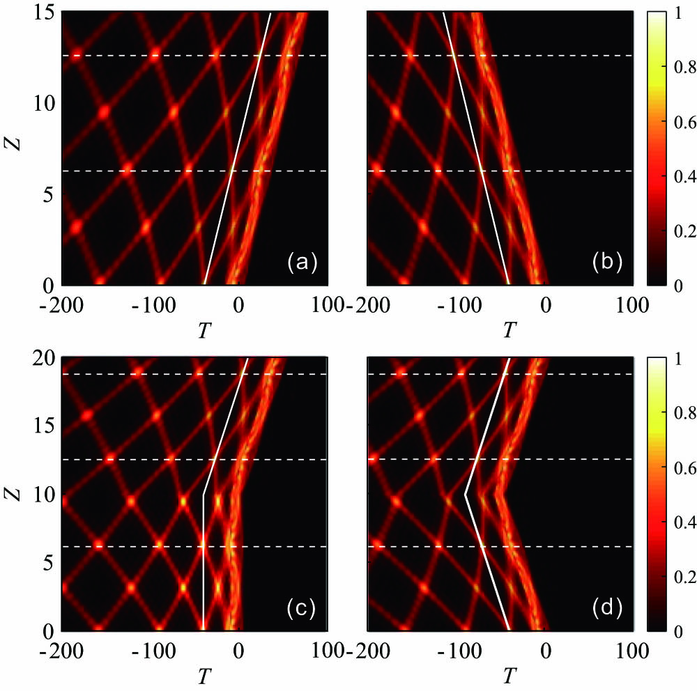
Fig. 2. (a), (b) Airy–Talbot effects of linearly chirped Airy pulse trains with C = 5 and C = −5, respectively. (c) Refractive Airy–Talbot effect. The input field at Z = 0 is unchirped and then linearly chirped with C = 5 at Z = 10. (d) Negative refractive Airy–Talbot effect. The input field at Z = 0 is linearly chirped with C = −5 and then chirped with C = 10 at Z = 10. The white solid line denotes the theoretical self-imaging trajectory. The self-imaging positions are marked by white dashed lines. Other parameters are the same as in Fig. 1(c).

Fig. 3. (a) Temporal evolution of the finite-energy Airy pulse train with a = 0.1. Other parameters are the same as in Fig. 1(c). (b) Same as (a) but for Δ = 8. (c) Maximal and minimal pulse separations to realize the Airy–Talbot effect for different truncation factors. The insets show CCC variations versus Z for Δ = 1.88 and 120 in the case of a = 0.02.

Fig. 4. (a) Temporal evolution of the input composed of stationary Airy pulses with a specific stretch factor of T₀ = (2α/k)^1/3. Here, we choose α = 1, and other parameters are the same as in Fig. 1. (b) Corresponding CCC variation with respect to Z. (c), (d) Same as (a) and (b) but for α = 2.

Fig. 5. (a) Temporal waveform of the input composed of two Airy pulses with δ = 2.588 and 3.882 in the case of α = −1. (b) Corresponding intensity pattern in the T–Z plane. (c), (d) Same as (a) and (b) but for α = 1. Here, we choose δ = −2.588 and −3.882. A = 1 and k = 1.