
Tianwen Han, Hao Chen, Wenwan Li, Bing Wang, Peixiang Lu. Temporal Airy–Talbot effect in linear optical potentials[J]. Chinese Optics Letters, 2021, 19(8): 082601
- Chinese Optics Letters
- Vol. 19, Issue 8, 082601 (2021)
Abstract
1. Introduction
The Talbot effect refers to the self-imaging phenomenon of a periodic paraxial optical field that was first, to the best of our knowledge, discovered by Talbot in 1836[
Recently, the Airy–Talbot effect was theoretically proposed and experimentally demonstrated in the spatial domain[
Given the space–time duality, the temporal Airy pulse has also been proposed and demonstrated[
Sign up for Chinese Optics Letters TOC. Get the latest issue of Chinese Optics Letters delivered right to you!Sign up now
In this work, we investigate the temporal Airy–Talbot effect in time-dependent linear potentials. We show that the accelerating self-imaging process can be enhanced or reduced by applying a linear potential, and the parabolic trajectory of self-imaging depends on both the dispersion sign and the linear potential gradient. By imposing linear phase modulations on the Airy pulse train, we realize the refractive Airy–Talbot effects with positive and negative refractions. For the stationary Airy pulse, having the form of an eigenfunction of the Schrödinger equation for a particle under a uniform force, the self-imaging follows straight lines, and the Airy–Talbot distance can be controlled by varying the linear potential gradient. The Airy–Talbot effect is also realized in the symmetric linear potential. All of the results can be extended to the spatial Airy beams, corresponding to the anomalous dispersion case here. The study provides a flexible approach to manipulate the Airy–Talbot effect and may find applications in optical communication and signal processing systems based on optical pulses.
2. Theoretical Model
The dynamics of optical pulses in a dispersive medium under a linear potential can be described by[
3. Results and Discussion
We first study the evolution of a linearly chirped self-accelerating Airy pulse train,
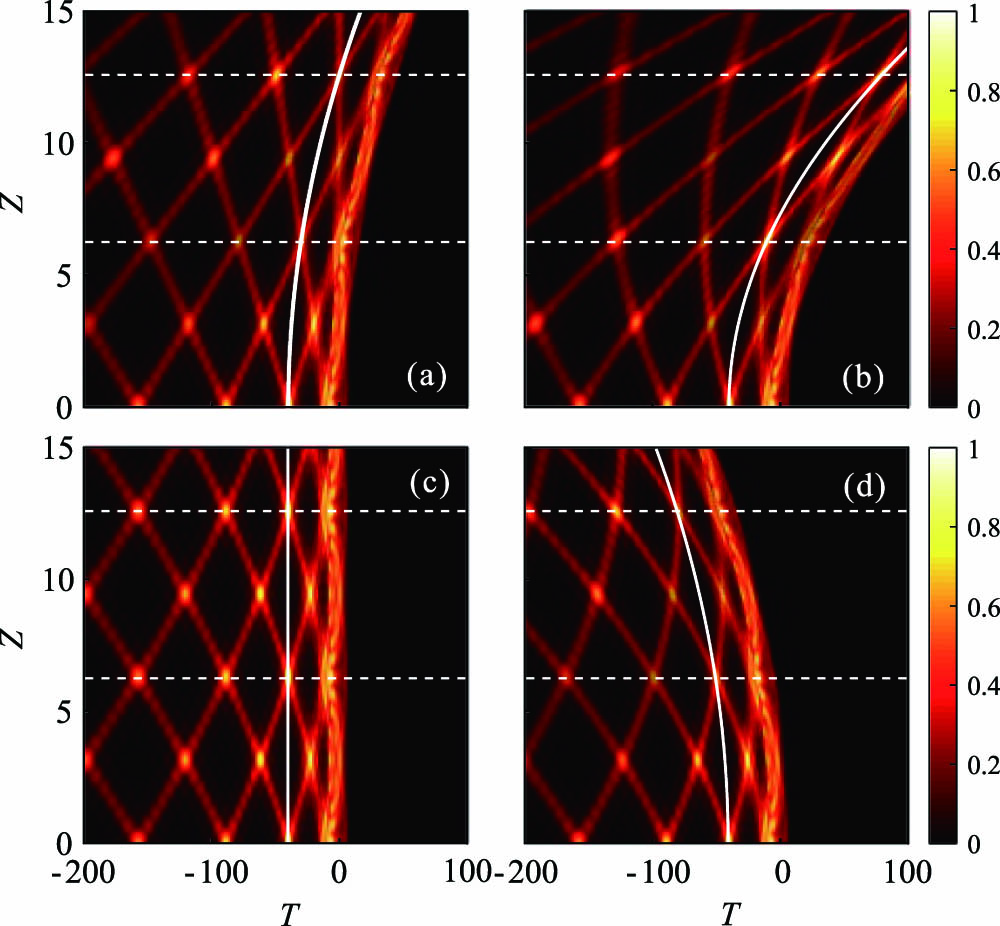
According to Eq. (3), each Airy pulse component has a different phase accumulation rate. Consequently, the initial intensity profile is reshaped during propagation as a result of interference between the Airy pulses. For ideal Airy pulse trains with , as the propagation distance satisfies the condition with being a nonzero integer, all of the Airy pulses are in phase. As a result, the input intensity pattern reproduces itself periodically along a modified parabolic trajectory in space–time. As , the trajectory takes the form of , which is determined by both the dispersion sign and the gradient of linear potential. In the absence of external potential, i.e., , the self-imaging trajectories in anomalous and normal dispersion regimes are identical. The Airy–Talbot distance is
To validate the above analysis, we numerically simulate the evolution of an Airy pulse train under the combined effects of dispersion and time-varying linear potential by using the split-step Fourier method[
![]()
Figure 1.Airy–Talbot effects for different linear potential gradients of (a) α = 0, (b) α = 1, (c) α = −1/2, and (d) α = −1. The white dashed lines indicate the first and second self-imaging positions. The white solid curve denotes the theoretical self-imaging trajectory. Parameters are a = 0, C = 0, k = 1, Δ = 2, cn = 1, and n ∈ [−3,3].
As the input pulse train is modulated by a linearly varying phase, the self-imaging trajectory follows the relation . The parabolic trajectory of self-images is similar to those of projectiles moving under the action of a uniform gravitational field, and plays the role of the initial launch velocity. If the intrinsic acceleration is restricted by the external linear potential, the self-imaging follows a straight line with the slope . Figure 2(a) shows the Airy–Talbot carpet of a linearly chirped Airy pulse train with , where the other parameters are the same as that in Fig. 1(c). The self-images are linearly shifted along the positive axis. On the contrary, the linearly chirped Airy pulse train with exhibits a mirror-symmetric evolution with respect to that of , as shown in Fig. 2(b). More interestingly, by imparting another linearly time-varying phase onto the pulse train during propagation, we can realize the refractive Airy–Talbot effect. In Fig. 2(c), the input pulse train is unchirped with and then modulated by a linearly varying phase with at . The white solid line denotes the theoretical self-imaging trajectory, which agrees well with the numerical results. In Fig. 2(d), the pulse train is first linearly modulated by at and then modulated by at , leading to an Airy–Talbot effect with negative refraction.
![]()
Figure 2.(a), (b) Airy–Talbot effects of linearly chirped Airy pulse trains with C = 5 and C = −5, respectively. (c) Refractive Airy–Talbot effect. The input field at Z = 0 is unchirped and then linearly chirped with C = 5 at Z = 10. (d) Negative refractive Airy–Talbot effect. The input field at Z = 0 is linearly chirped with C = −5 and then chirped with C = 10 at Z = 10. The white solid line denotes the theoretical self-imaging trajectory. The self-imaging positions are marked by white dashed lines. Other parameters are the same as in Fig.
The above analysis indicates that the input field composed of ideal Airy pulses can reproduce itself indefinitely. However, the ideal Airy pulses possess limitless time duration and infinite energy. In practice, we have to truncate the pulses so as to make them have finite energy. According to Eq. (3), the finite-energy Airy pulses (FEAPs) will experience dispersion, and the self-acceleration feature never maintains after the accelerating range, which is comparable to the dispersion length. Here, we choose , and the other parameters are the same as in Fig. 1(c). The temporal evolution of the pulse train is shown in Fig. 3(a), where the self-imaging effect disappears. The reason lies in the fact that the Airy–Talbot distance is beyond the accelerating range of FEAPs. In addition, the wave train propagates along a curved trajectory in the plane when is long enough, which is induced by the linear potential. By enlarging the pulse separation to , the self-imaging phenomenon appears, and the Airy–Talbot distance becomes , as shown in Fig. 3(b). For a fixed truncation factor, each Airy pulse has a specific accelerating range and time duration. To decrease the Airy–Talbot distance, we can enlarge the pulse separation between the FEAPs. The Airy–Talbot distance corresponding to the minimal pulse separation should be equal to the accelerating range. On the other hand, owing to the Airy–Talbot effect being a result of interference of overlapping Airy pulses, the maximal pulse separation should be less than the time duration of a single pulse. Figure 3(c) shows the numerical results of the allowable maximal and minimal pulse separations to realize the Airy–Talbot effect for different truncation factors. For , the maximal and minimal pulse separations are and , respectively. As increases, both the time duration and the accelerating range of each pulse decrease. Thus, the maximal pulse separation decreases, and the minimal one increases. As , the Airy–Talbot effect cannot be observed. Here, this value is obtained in the framework of a normalized pulse propagation equation. For the practical FEAPs with the main-lobe width , having the form of [
![]()
Figure 3.(a) Temporal evolution of the finite-energy Airy pulse train with a = 0.1. Other parameters are the same as in Fig.
Thus far, we have demonstrated that the parabolic self-imaging trajectory for the Airy–Talbot distance can be modified by the external linear potential. In fact, the stationary eigensolution of Eq. (1) is also an Airy wavefunction. Next, we show that the input field composed of stationary Airy pulses can produce self-images periodically along straight lines. Moreover, the Airy–Talbot distance can be tailored by varying the linear potential gradient. In this case, the input field reads
Unlike the above cases, the self-imaging is along straight lines regardless of the value of , and the Airy–Talbot distance becomes
The theoretical analysis can be verified by performing numerical simulations. Figure 4(a) shows the Airy–Talbot carpet for , where the other parameters are the same as in Fig. 1. The self-imaging is along straight lines, and the corresponding Airy–Talbot distance is . The white dashed lines in Fig. 4(a) denote the first and second self-imaging positions. The self-imaging effect can also be validated through CCC, which varies periodically with and reaches at (), as shown in Fig. 4(b). For , the Airy–Talbot distance becomes . The corresponding Airy–Talbot carpet and the CCC evolution with respect to are shown in Figs. 4(c) and 4(d), respectively. All results agree well with the theoretical predictions. Note that as , Eqs. (5)–(7) are reduced to Eqs. (2)–(4) for , respectively. Thus, the self-imaging shown in Fig. 1(c) is also along straight lines.
![]()
Figure 4.(a) Temporal evolution of the input composed of stationary Airy pulses with a specific stretch factor of T0 = (2α/k)1/3. Here, we choose α = 1, and other parameters are the same as in Fig.
Finally, we investigate the Airy–Talbot effect in symmetric linear potentials. The theoretical model can be described by
Figure 5(a) depicts the temporal profile of an input formed by the superposition of two Airy pulses with and 3.882 in the case of . Here, we choose and . The corresponding Airy–Talbot distance is . Figure 5(b) shows the Airy–Talbot carpet in the plane. The white dashed lines in Fig. 5(b) denote the two positions of and 9.71, at which the self-images are formed. Comparably, for , the Airy–Talbot effect in symmetric linear potential can also be obtained by choosing and . The corresponding temporal waveform of input is plotted in Fig. 5(c). The temporal evolution of input is shown in Fig. 5(d), where the Airy–Talbot distance is the same as that for .
![]()
Figure 5.(a) Temporal waveform of the input composed of two Airy pulses with δ = 2.588 and 3.882 in the case of α = −1. (b) Corresponding intensity pattern in the T–Z plane. (c), (d) Same as (a) and (b) but for α = 1. Here, we choose δ = −2.588 and −3.882. A = 1 and k = 1.
4. Conclusion
In summary, we have studied the Airy–Talbot effects of Airy pulse trains in time-dependent linear potentials. The parabolic space–time trajectory of self-imaging is determined by both the dispersion sign and the linear potential gradient. For the FEAPs, the effect can be observed only in a limited distance. The self-imaging trajectory can also be engineered by imposing linearly time-varying phases on the pulse train. For an input composed of stationary Airy pulses, the self-imaging follows straight lines, and the Airy–Talbot distance can be controlled by varying the linear potential gradient. The study provides a promising way to manipulate the self-imaging of aperiodic optical fields. The extension of the effects to other wave systems, such as Airy plasmons[
References
[1] H. F. Talbot. Facts relating to optical science. Philos. Mag., 9, 401(1836).
[2] J. Wen, Y. Zhang, M. Xiao. The Talbot effect: recent advances in classical optics, nonlinear optics, and quantum optics. Adv. Opt. Photon., 5, 83(2013).
[3] G. P. Agrawal. Nonlinear Fiber Optics(2013).
[4] J. Azaña, M. A. Muriel. Temporal Talbot effect in fiber gratings and its applications. Appl. Opt., 38, 6700(1999).
[5] R. Yang, Z. Xue, Z. Shi, L. Zhou, L. Zhu. Scalable Talbot effect of periodic array objects. Chin. Opt. Lett., 18, 030501(2020).
[6] Y. Lumer, L. Drori, Y. Hazan, M. Segev. Accelerating self-imaging: the Airy–Talbot effect. Phys. Rev. Lett., 115, 013901(2015).
[7] Y. Zhang, H. Zhong, M. R. Belić, X. Liu, W. Zhong, Y. Zhang, M. Xiao. Dual accelerating Airy–Talbot recurrence effect. Opt. Lett., 40, 5742(2015).
[8] Y. Zhang, H. Zhong, M. R. Belić, C. Li, Z. Zhang, F. Wen, Y. Zhang, M. Xiao. Fractional nonparaxial accelerating Talbot effect. Opt. Lett., 41, 3273(2016).
[9] G. A. Siviloglou, D. N. Christodoulides. Accelerating finite energy Airy beams. Opt. Lett., 32, 979(2007).
[10] G. A. Siviloglou, J. Broky, A. Dogariu, D. N. Christodoulides. Observation of Accelerating Airy beams. Phys. Rev. Lett., 99, 213901(2007).
[11] W. Liu, D. N. Neshev, I. V. Shadrivov, A. E. Miroshnichenko, Y. S. Kivshar. Plasmonic Airy beam manipulation in linear optical linears. Opt. Lett., 36, 1164(2011).
[12] Z. Ye, S. Liu, C. Lou, P. Zhang, Y. Hu, D. Song, J. Zhao, Z. Chen. Acceleration control of Airy beams with optically induced refractive-index gradient. Opt. Lett., 36, 3230(2011).
[13] X. Huang, Z. Deng, X. Fu. Dynamics of finite energy Airy beams modeled by the fractional Schrödinger equation with a linear potential. J. Opt. Soc. Am. B, 34, 3044(2017).
[14] S. Jia, J. Lee, J. W. Fleischer. Diffusion-trapped Airy beams in photorefractive media. Phys. Rev. Lett., 104, 253904(2010).
[15] N. K. Efremids. Airy trajectory engineering in dynamic linear index potentials. Opt. Lett., 36, 3006(2011).
[16] C.-Y. Hwang, K.-Y. Kim, B. Lee. Dynamic control of circular Airy beams with linear optical potentials. IEEE Photon. J., 4, 174(2012).
[17] H. Zhong, Y. Zhang, M. R. Belié, C. Li, F. Wen, Z. Zhang, Y. Zhang. Controllable circular Airy beams via dynamic linear potential. Opt. Express, 24, 7495(2016).
[18] G. G. Rozenman, M. Zimmermann, M. A. Efremov, W. P. Schleich, L. Shemer, A. Arie. Amplitude and phase of wave packets in a linear potential. Phys. Rev. Lett., 122, 124302(2019).
[19] X. Yan, L. Guo, M. Cheng, S. Chai. Free-space propagation of autofocusing Airy vortex beams with controllable intensity gradients. Chin. Opt. Lett., 17, 040101(2019).
[20] Y. Zhang, B. Wei, S. Liu, P. Li, X. Chen, Y. Wu, X. Dou, J. Zhao. Circular Airy beams realized via the photopatterning of liquid crystals. Chin. Opt. Lett., 18, 080008(2020).
[21] K. Zhan, Z. Yang, B. Liu. Trajectory engineering of Airy–Talbot effect via dynamic linear potential. J. Opt. Soc. Am. B, 35, 3044(2018).
[22] K. Zhan, J. Wang, R. Jiao, Z. Yang, B. Liu. Self-imaging effect based on circular Airy beams. Ann. Phys., 531, 1900293(2019).
[23] K. Zhan, R. Jiao, J. Wang, W. Zhang, Z. Yang, B. Liu. Self-imaging effect based on Airy beams with quadratic phase modulation. Ann. Phys., 532, 1900546(2020).
[24] Z. Li, P. Zhang, X. Mu, P. Jia, Y. Hu, Z. Chen, J. Xu. Guiding and routing of a weak signal via a reconfigurable gravity-like potential. Photon. Res., 7, 1087(2019).
[25] P. Jia, Z. Li, Y. Hu, Z. Chen, J. Xu. Visualizing a nonlinear response in a Schrödinger wave. Phys. Rev. Lett., 123, 234101(2019).
[26] I. Kaminer, Y. Lumer, M. Segev, D. N. Christodoulides. Causality effects on accelerating light pulses. Opt. Express, 19, 23132(2011).
[27] T. Han, B. Wang, P. Lu. Accelerating self-imaging effect for Airy pulse trains. Phys. Rev. A, 99, 053807(2019).
[28] M. Miyagi, S. Nishida. Pulse spreading in a single-mode fiber due to third-order dispersion. Appl. Opt., 18, 678(1979).
[29] C. Ament, P. Polynkin, J. V. Moloney. Supercontinuum generation with femtosecond self-healing Airy pulses. Phys. Rev. Lett., 107, 243901(2011).
[30] C.-C. Chang, H. P. Sardesai, A. M. Weiner. Dispersion-free fiber transmission for femtosecond pulses by use of a dispersion-compensating fiber and a programmable pulse shaper. Opt. Lett., 23, 283(1998).
[31] T. Han, H. Chen, C. Qin, W. Li, B. Wang, P. Lu. Airy pulse shaping using time-dependent power-law potentials. Phys. Rev. A, 97, 063815(2018).
[32] A. Banerjee, S. Roy. Trajectory manipulation of an Airy pulse near zero-dispersion wavelength under a free-carrier-generated linear potential. Phys. Rev. A, 100, 053816(2019).
[33] S. Wang, D. Fan, X. Bai, X. Zeng. Propagation dynamics of Airy pulses in optical fibers with periodic dispersion modulation. Phys. Rev. A, 89, 023802(2014).
[34] N. K. Efremidis, D. G. Papazoglou, S. Tzortzakis. Linear and nonlinear waves in surface and wedge index potentials. Opt. Lett., 37, 1874(2012).

Set citation alerts for the article
Please enter your email address
© Copyright 2018-2021 | Chinese Laser Press. All Rights Reserved 沪ICP备15018463号-20