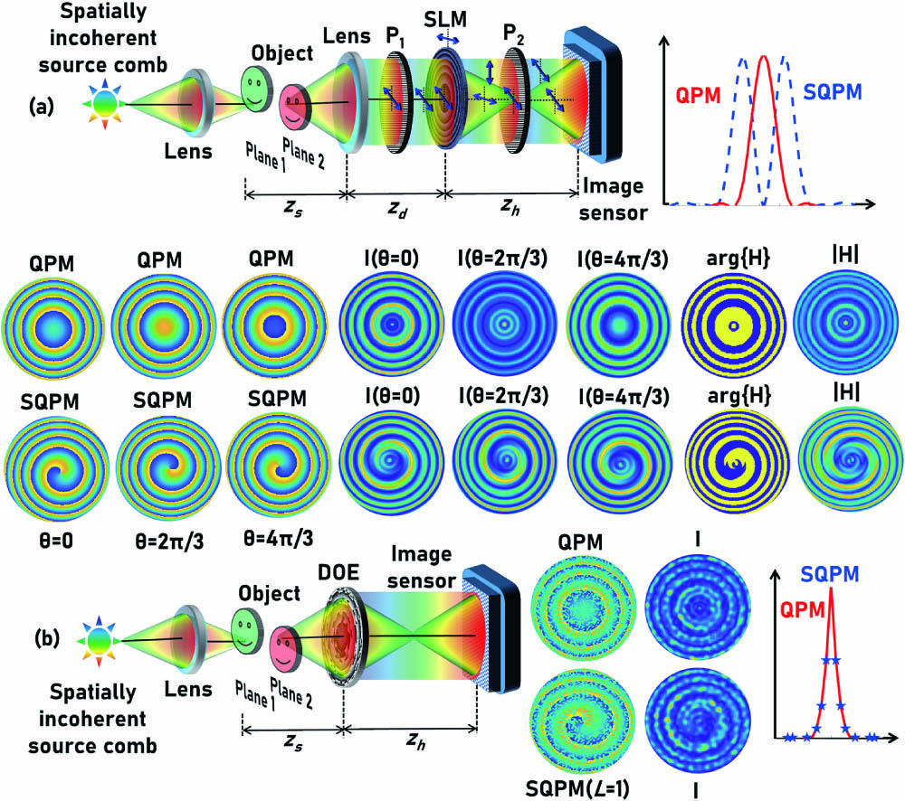
Fig. 1. Optical configuration of FINCH with (a) polarization multiplexing and (b) spatial multiplexing.

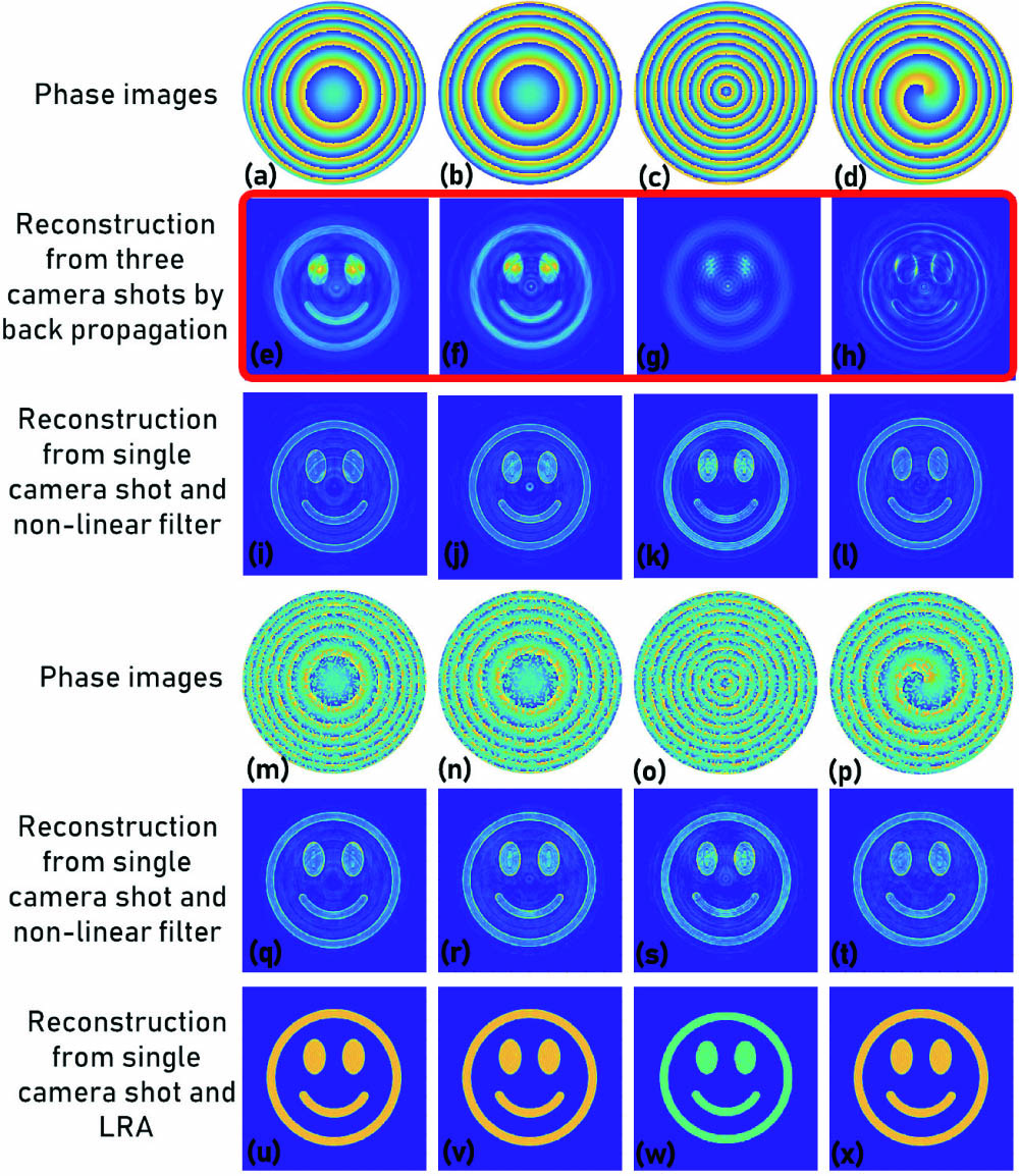
Fig. 2. Phase images of (a) QPM, (b) axilens, (c) axicon, and (d) SQPM. Reconstruction results of FINCH in the polarization multiplexing scheme with three camera shots and by back propagation for (e) QPM, (f) axilens, (g) axicon, and (h) SQPM. Reconstruction results of FINCH in the polarization multiplexing scheme with a single camera shot and non-linear correlation for (i) QPM, (j) axilens, (k) axicon, and (l) SQPM. Phase images of randomly multiplexed constant matrix and (m) QPM, (n) axilens, (o) axicon, and (p) SQPM. Reconstruction results of FINCH in the spatial multiplexing scheme with non-linear correlation for (q) QPM, (r) axilens, (s) axicon, and (t) SQPM. Reconstruction results of FINCH in the spatial multiplexing scheme with a single camera shot and LRA for (u) QPM, (v) axilens, (w) axicon, and (x) SQPM.

Fig. 3. Plot of I(x = 0, y = 0) for FINCH (QPM), FINCH (axicon), and direct imaging for variation in the object distance z_s (0.1 to 0.3 m) for FINCH1, reconstruction by back propagation, and FINCH2, reconstruction by cross correlation.

Fig. 4. (a) Gerchberg–Saxton algorithm and generated phase masks with (b) σ=0.5, (c) σ=0.1, (d) σ=0.04, and (e) σ=0.02.

Fig. 5. Plot of I(x = 0, y = 0) for (a) FINCH (QPM) and (b) FINCH (axicon) with spatial multiplexing and non-linear correlation for variation in the object distance z_s (0.1 to 0.3 m) for different scattering ratios σ=0.02, 0.04, 0.1, and 0.5.

Fig. 6. Optical microscope images of randomly multiplexed (a) QPMs and (b) the QPM and axicon.

Fig. 7. Plot of the logarithm of the cross-correlation value for variation in distance from z_s = 5 cm. The holograms recorded at z_s = 5.2 cm, 5.4 cm, 5.7 cm, and 6 cm are shown.