
Xiangyu Pei, Xunbo Yu, Xin Gao, Xinhui Xie, Yuedi Wang, Xinzhu Sang, Binbin Yan. End-to-end optimization of a diffractive optical element and aberration correction for integral imaging[J]. Chinese Optics Letters, 2022, 20(12): 121101
- Chinese Optics Letters
- Vol. 20, Issue 12, 121101 (2022)
Abstract
Keywords
1. Introduction
Three-dimensional (3D) display technology is capable of providing real and natural 3D perception, and, consequently, various efforts have been made to advance this technology further[
Despite numerous advantages, the widespread application of the II method is limited because of several factors such as low viewing resolution, narrow viewing angle, and shallow depth of field (DOF)[
In this paper, an end-to-end joint optimization method for optical components and image input sources is proposed. In this method, first, a DOE model is established in the form of thickness variables and combined with the wave optics imaging model to derive the light intensity distribution of the point light source passing through the element at the imaging plane. Second, the deep learning network is employed to pre-correct the input image, and the derived light intensity distribution is subsequently used to simulate the display image of the pre-corrected image on the imaging surface, through the DOE. Finally, the element images (EIs) in the SI are used as the training dataset, and the stochastic gradient method is used to jointly optimize the aforementioned two parts. In summary, when designing the surface parameters of the DOE, the deep learning network is used to pre-correct the EIA to overcome the aberration problem. Because the light intensity distribution formed at different positions on the input plane is different, the processing method of dividing multiple fields of view—the images in different fields of view are convoluted with the corresponding point spread function (PSF) to simulate the display image of the pre-corrected image at the imaging plane after passing through the DOE—was adopted in this study. The experimental results showed that by using this method the surface parameters of the DOE can be optimized, which effectively mitigates the aberration problem and aids in achieving a highly accurate display result of the original image.
Sign up for Chinese Optics Letters TOC. Get the latest issue of Chinese Optics Letters delivered right to you!Sign up now
2. End-to-End Optimization Method
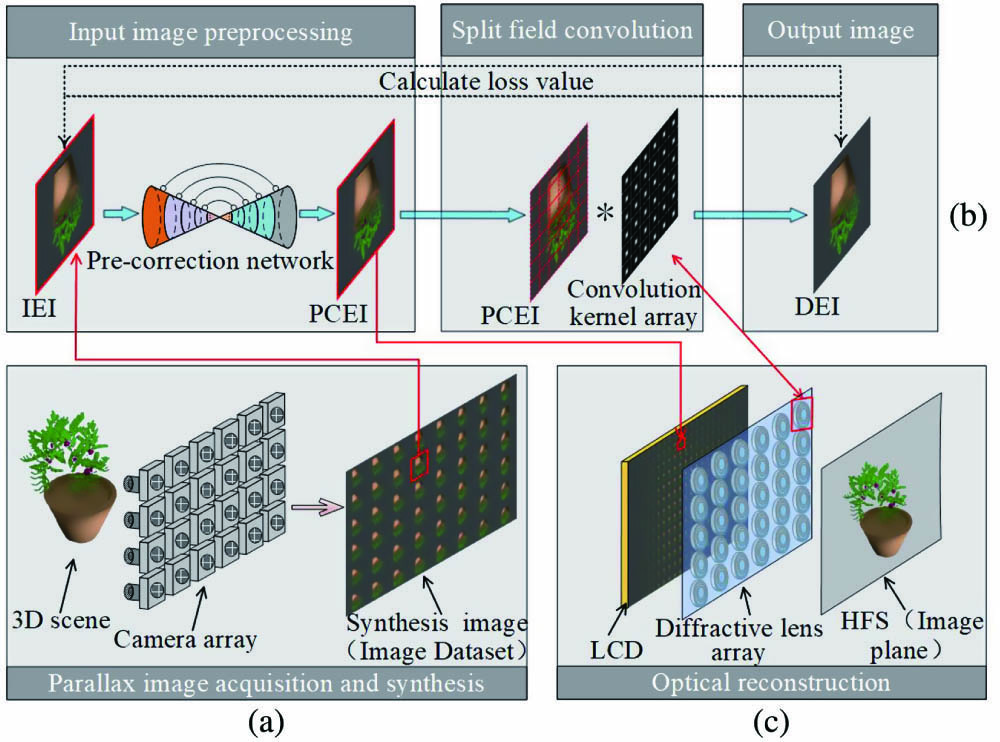
The proposed end-to-end optimization of the DOE and aberration correction consists of three steps: (i) input image pre-correction stage, (ii) pre-corrected image subfield convolution stage, and (iii) loss calculation stage, as shown in Fig. 1(b). Figure 1(a) shows the information acquisition stage in the II display method. The camera array collects information from different angles of the 3D scene and encodes it into an SI, which is composed of an EIA. The EIA is used as the training dataset, and each EI is used as the input source to enter the closed-loop process of the method shown in Fig. 1(b). Then, the trained DOE is repeatedly arranged to form a diffractive LA, and the trained pre-correction EI (PCEI) is loaded on the display panel, as shown in Fig. 1(c). In the input image pre-correction stage, the input EI (IEI) passed through the deep learning pre-correction network to obtain the PCEI. Next, the PCEI enters as the input to the pre-corrected image subfield convolution stage, where the input image is divided into multiple regions, and each region image is convolved with its corresponding PSF convolution kernel to simulate the final display EI (DEI). Finally, by calculating the loss value between the DEI and the IEI, the surface parameters of the DOE and PCEI are obtained via back propagation.
![]()
Figure 1.Overall workflow diagram of this experiment: (a) parallax image acquisition and synthesis; (b) proposed end-to-end optimization method workflow; and (c) optical reconstruction.
2.1. Image display model
The ideal optical system differs significantly from the actual optical system. After passing through the actual optical system, the light emitted from an object point in the object space does not converge to a point in the image space; instead, it forms a diffused spot, as shown in Fig. 2. The size of the diffused spot is governed by the aberration of the system. In wave optics theory, ideally, the spherical wave emitted by an object point remains a spherical wave after passing through the optical system. Because of diffraction, the ideal image of an object point is a complicated Airy disk. However, in the actual optical system, because of aberration, the wave surface formed by the optical system does not remain a spherical surface, but exhibits a certain wave phase difference. As a result of aberration, the original input image (OII), after passing through the optical system, becomes distorted, resulting in a different display image. Mathematically, the point light source can be represented by the function (point pulse). For an optical system, the light field intensity distribution of the point imaged by the point light source is called the PSF. The image formed by the optical system is a result of the convolution of the object image and the PSF of each point. To simulate the display results, we derive a wave-based image display model, which incorporates the diffraction-related effects on the display. The derived image display model is based on Fourier optics, and we have effectively integrated it into the workflow of the deep learning tools.
![]()
Figure 2.Imaging process of an actual optical system.
To derive the PSF of an optical element, we model the spherical wave emitted by the point light source on a liquid crystal display (LCD) plane and then calculate the wave field expression when it passes through the DOE and subsequently reaches the HFS.
As shown in Fig. 3, the plane where the LCD located is described by a 2D coordinate system , on which a point light source, with an initial amplitude and initial phase of and , respectively, reaches the left surface of the DOE (the plane described by the 2D coordinate system ). Based on wave optics theory, the wave expression of the point light source on the left surface of the DOE is given by (assuming )
![]()
Figure 3.Schematic diagram of the light intensity distribution at different field points on the image plane.
For a single refractive or DOE such as a thin lens, the delay of the wave field phase is proportional to the thickness at the corresponding position, and the amplitude of the wave field shows negligible changes, i.e.,
The wave field , with an amplitude of and a phase of , is incident on the optical element, and, after passing through the element, it changes to
As shown in Fig. 3, the wave field reaches the HFS (the plane is described by the 2D coordinate system ) after propagating a distance in free space. The wave field expression at this plane can be expressed as
This formula uses the Fresnel propagation operator; when , Eq. (4) yields an accurate model for near and far distances. The PSF [] is given by the square of the magnitude of the complex-valued wave field, i.e., , as
Equations (1) to (5) show that the PSF value is related to wavelength. Considering that the pixels on the display panel are composed of subpixels of red, green, and blue colors, we input the PSF corresponding to these three colors into the end-to-end network. In network optimization learning, on the one hand, the surface shape of the DOE can be optimized; on the other hand, the input image can be pre-corrected to adapt to the surface shape of the DOE so that both chromatic aberration and geometric aberration can be taken into account.
In addition, from the derivation process of the formula, it can be seen that the light intensity distribution formed by the point sources at different positions on the object surface on the HFS is different. As shown in Fig. 3, the PSF convolution kernels corresponding to the three point sources at different positions are different. For obtaining a more realistic simulation display result, we evenly divide the input image into regions, and each subregion is denoted by . The light intensity distribution formed by each point in the subregion, after passing through the optical element, can be approximated by its central point, whose PSF is denoted by . The image formed by the subregion , through the optical system, is denoted by , which can be described by the convolution of and as
Using this formula, the display result, CI, of the input image, after passing through the DOE, can be obtained as
2.2. Pre-correction network
In this study, a network structure was built for the pre-correcting input image and subsequently used to preprocess the original image loaded on the display panel. Further, this developed network structure was used to calculate the parameters of the deep learning network and the surface parameters of the DOE jointly. The proposed network structure consists of two parts: the recognition network and the generation network, as shown in Fig. 4. The recognition network reduces the image size and extracts some simple features through convolution and down sampling, while the generation network obtains some deep features through convolution and up sampling. In addition, to make full use of the feature information and retain the richer scene details, we superimpose the feature information on the recognition network and generated network path.
![]()
Figure 4.Pre-correction network structure.
Specifically, each layer of the recognition network is composed of a convolutional layer for down sampling (stride: 2; size: ), a batch normalization (BN) layer for preprocessing the data, and a leaky rectified linear unit (LeakyReLU) activation function. In each down sampling convolution, we reduce the size of the feature map by half and double the number of feature channels. Due to the data diversity of the 3D scene, the BN layer can ensure that the data of each layer is passed down within an effective range, and the LeakyReLU activation function allows the loss signal to be propagated back to the previous layer. Each layer of the generation network consists of a transposed convolutional layer (step size: 2; size: ) for up sampling, a BN layer for preprocessing the data, and a ReLU activation function. In each up sampling convolution, we double the size of the feature map and reduce the number of feature channels by half.
2.3. Overall loss function
Initially, the OII is obtained through the pre-corrected image network proposed and described in section 2.2 to extract the pre-corrected image. Subsequently, the final display image can be calculated using the image display model derived in Section 2.1. The traditional neural network usually uses the mean square error (MSE)[
3. Experiment and Simulation Results
The aperture diameter, focal length, and F-number of the optical element designed in the experiment are 5 mm, 19.23 mm, and 3.85, respectively. The optical element is discretized with a 12.63 µm feature size on a grid. Rotational symmetry is considered in the design of diffractive elements. Although our method can be generalized to rotational asymmetric shapes, rotational symmetry is helpful for manufacturing using turning machines. In order to more accurately construct 3D display spatial voxels and improve light energy utilization, positive first-order diffraction light was selected.
The experiment was carried out according to the workflow shown in Fig. 1, and the experimental parameters are shown in Table 1. First, a virtual camera array is used to capture information from different directions of the 3D scene to develop the 3D model. The LA in the 3D reproduction stage consists of lens units. According to the designed light field display system parameters, the SI of the 3D model can be obtained, i.e., the SI contains EIs. These EIs become the training dataset in this experiment. We choose the Momentum optimizer with , which exhibits robustness to our image dataset. Considering the parameters updating speed and preventing the parameters from hovering near the optimal value, we choose the learning rate of polynomial decay. When the starting learning rate and end learning rate were and , respectively, the training effect of network on our image dataset was better.
| Parameters | Values |
|---|---|
| Aperture diameter | 5 mm |
| Light source distance (zo) | 20 mm |
| Propagation distance (d) | 500 mm |
| Focal length | 19.23 mm |
| F number | 3.85 |
| Number of training dataset images | |
| Number of image subregions |
Table 1. Optical Element and Image Dataset Parameters
In the image subfield convolution stage, we divide the pre-corrected EI into subregions (as shown in Fig. 5), and the corresponding PSF convolution core array also contains PSF convolution cores. The sampling point of each PSF convolution core is consistent with the resolution of the subregion image. The experimental DOE and loss curve obtained during the training using the proposed end-to-end framework are shown in Figs. 6(a) and 6(b), respectively. The experimental DOE and loss curve obtained during the training without using the pre-correction network are shown in Figs. 7(a) and 7(b), respectively. Due to the rotational symmetry of the lens unit, Figs. 6(c) and 7(c) show the logarithm of nine of the PSF convolution kernels (corresponding to the nine subregions marked in Fig. 5).
![]()
Figure 5.All 36 subsections of an EI and its corresponding diffractive lens unit.
![]()
Figure 6.Experimental results with end-to-end optimization: (a) diffractive element profile; (b) loss curve during training; and (c) PSF of nine fields of view, in logarithmic scale.
![]()
Figure 7.Experimental results without pre-correction network: (a) diffractive element profile; (b) loss curve during training; and (c) PSF of nine fields of view, in logarithmic scale.
To verify the effectiveness of the proposed end-to-end joint optimization framework, we conducted optical simulation experiments. As shown in Fig. 8, the simulation experiments were carried out from five different observation positions: central position, above, below, left, and right. Figures 8(a)–8(c) display the image of the original scene, simulation results without using the pre-correction network, and simulation results with end-to-end optimization, respectively. As evident from the enlarged images shown in Figs. 8(b) and 8(c), the experimental results optimized by the end-to-end method as well as the display quality are significantly improved. In addition, the peak signal to noise ratio (PSNR) value is significantly improved, which proves the effectiveness of the framework.
![]()
Figure 8.Simulation results for different viewing positions (with multiple PSFs): (a) original scene; (b) simulation results without pre-correction network; and (c) simulation results with end-to-end optimization.
To demonstrate the effectiveness of dividing the field of view to employ multiple PSFs, we supplemented a comparative simulation experiment using a single PSF, and the simulation results are shown in Fig. 9. When using a single PSF approximation, it can be seen from Fig. 9 that only the simulation results from the center viewpoint are better, and this difference will gradually accumulate as the viewing angle increases. Furthermore, the experimental results shown in Fig. 9 are better than those shown in Fig. 8 with or without the use of the pre-correction network, which shows that dividing the field of view to employ multiple PSFs is the correct choice.
![]()
Figure 9.Simulation results for different viewing positions (with a single PSF): (a) original scene; (b) simulation results without pre-correction network; and (c) simulation results with end-to-end optimization.
The optical aberrations of the proposed design have the following properties. The chromatic variation is small because the deep diffraction lens surface [as shown in Fig. 6(a)] obtained by using end-to-end frame optimization results in only small focal length differences in the visible wavelength region. In addition, the diffraction lenses also interact with each other, which is taken into account in our design. Similar to the traditional optical LA, the 3D optical field display system based on the diffraction LA will form multiple view areas in space. We form the region of interaction between diffraction lenses outside the visible region to ensure the purity of spatial voxels in the visible region.
One possible solution similar to diffraction lenses is metalenses, which have recently enabled the fabrication of single ultrathin optical elements that encode wavelength-dependent phase patterns onto the incoming light. There is a recent paper[
4. Conclusion
In this paper, we propose and introduce an end-to-end joint optimization method for DOE and for preprocessing input images. The method mainly includes two steps. In the first step, we establish a DOE model, derive the light intensity distribution of point light sources, from different fields of view, at the imaging surface based on wave optics theory, and obtain the corresponding PSF convolution kernel array. In the second step, we build a pre-corrected image network to preprocess the input image and load the preprocessed image onto the display panel. Finally, combining the MSE and SSIM loss functions and employing the EIs that form the SIs as the training dataset, we jointly calculate the surface parameters of the DOE, the parameters of the pre-corrected image network, and the pre-processed image. The surface parameters of the DOE as well as the PSF of the sampling points, extracted from different fields of view, are obtained through this method. The simulation results show that the end-to-end joint optimization method effectively reduces the aberration problem and significantly improves the quality of the display image.
References
[1] G. J. Lv, Q. H. Wang, W. X. Zhao, J. Wang. 3D display based on parallax barrier with multiview zones. Appl. Opt., 53, 1339(2014).
[2] N. Okaichi, M. Miura, J. Arai, M. Kawakita, T. Mishina. Integral 3D display using multiple LCD panels and multi-image combining optical system. Opt. Express, 25, 2805(2017).
[3] S. Xing, X. Sang, X. Yu, C. Duo, B. Pang, X. Gao, S. Yang, Y. Guan, B. Yan, J. Yuan, K. Wang. High-efficient computer-generated integral imaging based on the backward ray-tracing technique and optical reconstruction. Opt. Express, 25, 330(2017).
[4] J. Y. Son, C. H. Lee, O. O. Chernyshov, B. R. Lee, S. K. Kim. A floating type holographic display. Opt. Express, 21, 20441(2013).
[5] W. Song, Q. Zhu, Y. Liu, Y. Wang. Volumetric display based on multiple mini projectors and a rotating screen. Opt. Eng., 54, 013103(2015).
[6] X. Sang, F. C. Fan, C. C. Jiang, S. Choi, W. Dou, C. Yu, D. Xu. Demonstration of a large-size real-time full-color three-dimensional display. Opt. Lett., 34, 3803(2009).
[7] N. Balram, I. Tosic. Light-field imaging and display systems. Inf. Disp., 32, 2(2016).
[8] R. Bregović, P. T. Kovács, A. Gotchev. Optimization of light field display-camera configuration based on display properties in spectral domain. Opt. Express, 24, 3067(2016).
[9] H. Huang, H. Hua. Systematic characterization and optimization of 3D light field displays. Opt. Express, 25, 18508(2017).
[10] G. Lippmann. La photographie integrale. C. R. Acad. Sci., 146, 446(1908).
[11] J. H. Park, Y. Kim, J. Kim, S. W. Min, B. Lee. Three-dimensional display scheme based on integral imaging with three dimensional information processing. Opt. Express, 12, 6020(2004).
[12] J.-S. Jang, F. Jin, B. Javidi. Three-dimensional integral imaging with large depth of focus by use of real and virtual image fields. Opt. Lett., 28, 1421(2003).
[13] J.-S. Jang, B. Javidi. Depth and lateral size control of three-dimensional images in projection integral imaging. Opt. Express, 12, 3778(2004).
[14] J.-S. Jang, B. Javidi. Large depth of focus time-multiplexed three-dimensional integral imaging by use of lenslets with nonuniform focal lens and aperture sizes. Opt. Lett., 28, 1924(2003).
[15] R. Martínez-Cuenca, G. Saavedra, M. Martínez-Corral, B. Javidi. Extended depth-of-field 3-D display and visualization by combination of amplitude-modulated microlenses and deconvolution tools. J. Display Technol., 1, 321(2005).
[16] R. Martínez-Cuenca, G. Saavedra, M. Martínez-Corral. Enhanced depth of field integral imaging with sensor resolution constraints. Opt. Express, 12, 5237(2004).
[17] L. Erdmann, K. J. Gabriel. High resolution digital integral photography by use of a scanning microlens array. Appl. Opt., 40, 5592(2001).
[18] S. Kishk, B. Javidi. Improved resolution 3D object sensing and recognition using time multiplexed computational integral imaging. Opt. Express, 11, 3528(2003).
[19] J. S. Jang, B. Javidi. Three-dimensional synthetic aperture integral imaging. Opt. Lett., 27, 1144(2002).
[20] J. S. Jang, B. Javidi. Improved viewing resolution of three-dimensional integral imaging by use of nonstationary micro-optics. Opt. Lett., 27, 324(2002).
[21] S. Banerji, B. Sensale-Rodriguez. A computational design framework for efficient, fabrication error-tolerant, planar THz diffractive optical elements. Sci. Rep., 9, 5801(2019).
[22] S. Banerji, M. Meem, A. Majumder, F. G. Vasquez, B. Sensale-Rodriguez, R. Menon. Imaging with flat optics: metalenses or diffractive lenses?. Optica, 6, 805(2019).
[23] M. Meem, S. Banerji, C. Pies, T. Oberbiermann, A. Majumder, B. Sensale-Rodriguez, R. Menon. Large-area, high-numerical-aperture multi-level diffractive lens via inverse design. Optica, 7, 252(2020).
[24] S. Banerji, M. Meem, A. Majumder, B. Sensale-Rodriguez, R. Menon. Extreme-depth-of-focus imaging with a flat lens. Optica, 7, 214(2020).
[25] P. Wang, N. Mohammad, R. Menon. Chromatic aberration corrected diffractive lenses for ultra broadband focusing. Sci. Rep., 6, 21545(2016).
[26] N. Antipa, G. Kuo, R. Heckel, B. Mildenhall, E. Bostan, R. Ng, L. Waller. DiffuserCam: lensless single-exposure 3D imaging. Optica, 5, 1(2018).
[27] M. S. Asif, A. Ayremlou, A. Veeraraghavan, R. Baraniuk, A. Sankaranarayanan. Flatcam: replacing lenses with masks and computation. IEEE International Conference on Computer Vision (ICCV), 663(2015).
[28] Y. Peng, Q. Sun, X. Dun, G. Wetzstein, W. Heidrich. Learned large field-of-view imaging with thin-plate optics. ACM Trans. Graph., 38, 219(2019).
[29] K. Monakhova, J. Yurtsever, G. Kuo, N. Antipa, K. Yanny, L. Waller. Learned reconstructions for practical mask-based lensless imaging. Opt. Express, 27, 28075(2019).
[30] V. Sitzmann, S. Diamond, Y. Peng, X. Dun, S. Boyd, W. Heidrich, F. Heide, G. Wetzstein. End-to-end optimization of optics and image processing for achromatic extended depth of field and super-resolution imaging. ACM Trans. Graph., 37, 114(2018).
[31] A. Nikonorov, V. Evdokimova, M. Petrov, P. Yakimov, S. Bibikov, Y. Yuzifovich, R. Skidanov, N. Kazanskiy. Deep learning-based imaging using single-lens and multi-aperture diffractive optical systems. IEEE/CVF International Conference on Computer Vision Workshop (ICCVW), 3969(2019).
[32] E. Bauer, R. Kohavi. An empirical comparison of voting classification algorithms: bagging, boosting, and variants. Mach. Learn., 36, 105(1999).
[33] Z. Wang, A. Bovik, H. R. Sheikh, E. P. Simoncelli. Image quality assessment: from error visibility to structural similarity. IEEE Trans. Image Process., 13, 600(2004).
[34] E. Tseng, S. Colburn, J. Whitehead, L. Huang, S.-H. Baek, A. Majumdar, F. Heide. Neural nano-optics for high-quality thin lens imaging. Nat. Commun., 12, 6493(2021).

Set citation alerts for the article
Please enter your email address
© Copyright 2018-2021 | Chinese Laser Press. All Rights Reserved 沪ICP备15018463号-20