It is always an important subject that the accurate measurement of key parameters in fields of manufacturing. The measuring accuracy of the outer diameter directly determines the assemble efficiency and products’ quality^[1]. The diameter is traditionally performed by micrometer, caliper gauge, and other telescopic mechanical tools^[2-3]. In addition, the coordinate measuring machine (CMM) can undertake the dimension measurement tasks due to its high measurement accuracy and advanced technology^[4-6]. However, the costs and measurement efficiency restricts the wide use of coordinate measuring machine^[7]. To meet these requirements, the laser measurement plays is applied in the field of non-contact measurement due to its high precision and convenience^[8].

In the numerous method of diameter measurement methods, the three-point method is widely applied in the precision machining because of the high accuracy and small errors, which is one of the important technical components of the manufacturing industry^[9]. Aoki Yasuo first proposed the separation technique of roundness errors by in 1966. Basing on the frequency domain method of Fourier transform, the algorithm invloved a disadvantage of the loss of frequency components that the transfer function’s denominator is zero^[10-11]. A three-point method of three parallel displacement sensors was proposed by Hong Maisheng and he developed a algorithm which separate roundness errors and rotation errors successfully^[12-13]. But the problem of haemonic suppression was not solved because of the angle setting errors. And in the percision measurement of diameters, little error can cause enormous deviation. So the angle setting errors has to be calibrated before measurement.

This paper studies a new model which is about angle setting errors of the diameter measurement based on three-point method, including the calibration and the experiment. According to the principle of a settled circle which is determined by three points not on the same straight line, we developed an outer diameter measuring system with three laser displacement sensors. The sensor is based on the laser triangulation method, which mainly uses the reflected and scattered beams of laser to accept the information of the target surface or distances between different targets^[14], which is widely used in the measurement of length and distance in industry^[15]. As for the three-point method, we do the simulation about angle setting errors and study their influences. Finally, we design and assemble the experimental device to confirm the effectiveness of the calibration. The main purposes of this paper are to put forward a scheme of calibration based on the least squares and the iterative method and to calibrate the angle setting errors. After the calibration, the outer diameter measurement device can independently measure the workpiece and extremely increase the accuracy of measurement.

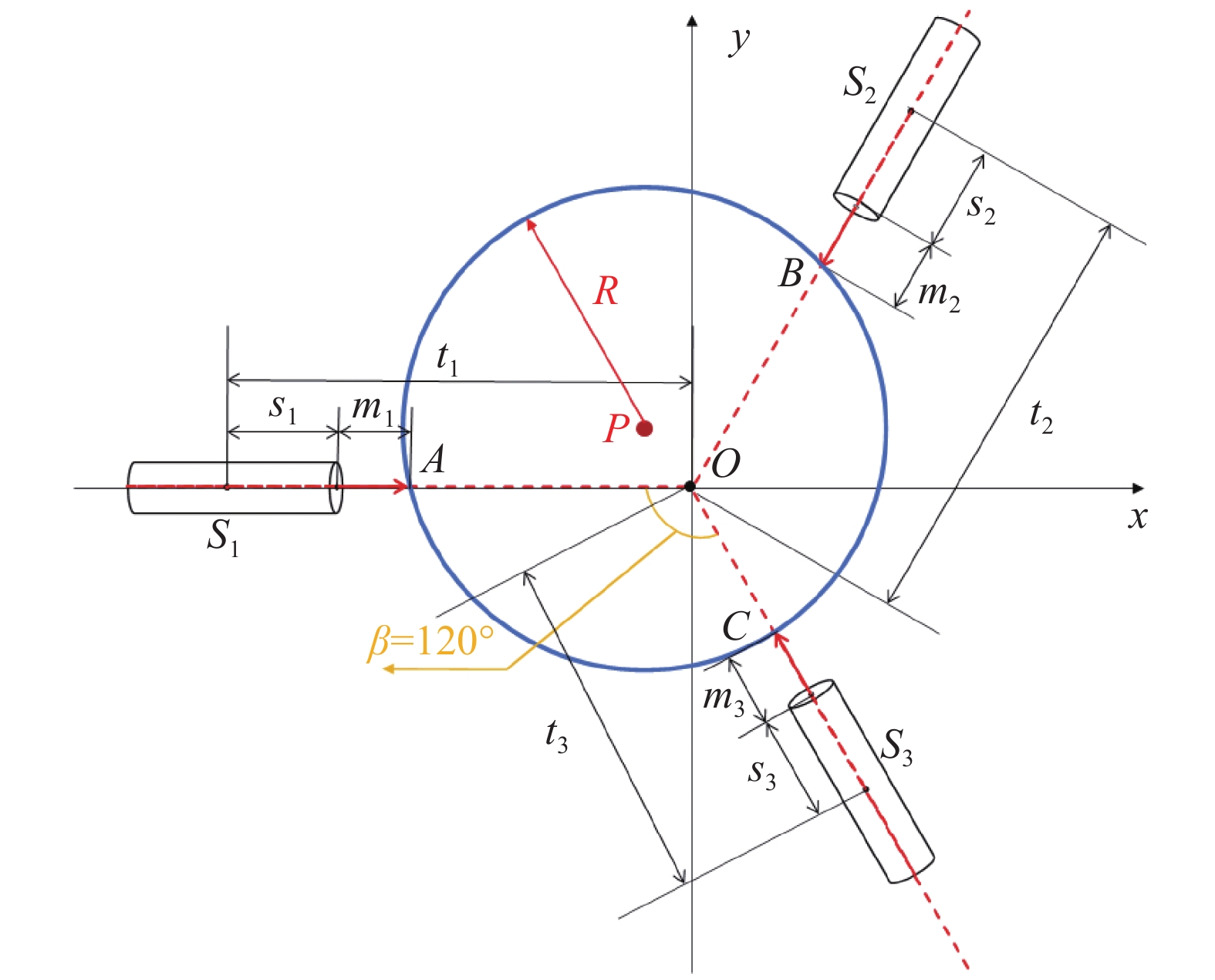
The basic principle of three-point method is to set the three sensors at a fixed angle, such as 120°. The measurement axes of sensors intersect at one point. Then we can build the XOY coordinate system by taking the point as origin and get multiple sets of measurements when rotating the workpiece. At last, we calculate the diameter according to the coordinates of the three points on the circle. Figure1 illustrates the three-point method without considerations of the angle setting errors. Three sensors are 120° apart from each other along the measurement axis. O is the origin and P is the center of the circle. S is the rotation center of each displacement sensor. The coordinates of A, B and C (A_x, A_y, B_x, B_y, C_x, C_y) can be determined according to the measurements m₁, m₂ and m₃. Lastly, we can figure up the diameter and the position of P through the coordinates.

The calculation formula is as follows:

$\left\{ \begin{array}{l} {A_x} = - \left( {{t_1} - {s_1} - {m_1}} \right),{A_y} = 0\\ {B_x} = \dfrac{1}{2}({t_2} - {s_2} - {m_2}),{B_y} = \dfrac{{\sqrt 3 }}{2}({t_2} - {s_2} - {m_2})\\ {C_x} = \dfrac{1}{2}({t_3} - {s_3} - {m_3}),{C_y} = - \dfrac{{\sqrt 3 }}{2}({t_3} - {s_3} - {m_3}) \end{array} \right.$ (1)

As we can see from the Fig.1, s₁,s₂ and s₃ are the distances of the rotation center to the origin, t₁, t₂ and t₃ are the distances of the rotation center to the front end. s and t are never changed when the positions of sensors are settled. The radius r can be obtained by Eq.(2).

$\left\{ \begin{array}{l} {({P_x} - {A_x})^2} + {({P_y} - {A_y})^2} = {r^2} \\ {({P_x} - {B_x})^2} + {({P_y} - {B_y})^2} = {r^2} \\ {({P_x} - {C_x})^2} + {({P_y} - {C_y})^2} = {r^2} \\ \end{array} \right.$ (2)

Figure 2 shows the three-point method with considerations of angel setting errors. In this model, we think that there exist one fixed point in each sensor and the probe will occur a small deflection around the point. The sensor turns around point S, which means the center of rotation in the measurement. This is the theoretical basis of the calibration and simulation.

It is known from the principle of three-point method that the position of origin O is determined by rotation centers of three sensors. The positions of sensors are never changed and the aims of the measurements are to examine different workpieces’ diameters when we do the work in reality. So the position of O is settled by sensors and without errors. In addition, the fixed parameters are the distance s from the rotation center to the zero point of measurement, the distance t between O and S, and the angle setting error α in the model. The three parameters can be named as systemic parameters. And s and α are unknown to be calibrated. The measured value m and the position of circle are changed between different measurements. Therefore, sensors’ values m are the input; the output are coordinates of centers (P₁, P₂) and the radius r in the whole system. γ is the angle that after rotations. The specific relationship of the parameters can be calculated by Eq.(2) and (3):

$\left\{ \begin{array}{l} {A_x} = - [{t_1} - \left( {{s_1} + {m_1}} \right)]\cos {\gamma _1},{A_y} = (s_1 + m_1)\sin {\gamma _1}\\ {B_x} = [{t_2} - ({s_2} + {m_2})]\cos {\gamma _2},{B_y} = ({t_2} - {s_2} - {m_2})\sin {\gamma _2}\\ {C_x} = [{t_3} - ({s_3} + {m_3})]\cos {\gamma _3},{C_y} = - [{t_3} - ({s_3} + {m_3})]\sin {\gamma _3} \end{array} \right.$ (3)

Due to the nonlinearity of the equations, that we cannot get the analytical expression. Then we choose to use the least squares and the lterative method to do the calibration. Solving the Eq.(3), the forward kinematic solution P, the position of the workpiece and the radius in the coordinate system, is given by:

$ {{P}} = F({{M}},{ S})$ (4)

where M is the measured values and S is the systemic parameter vector as follows:

$ {{S}} = \mathop {\left[ {s_1\;s_2\;s_3\;\alpha _1\;\alpha _2\;\alpha _3} \right]}\nolimits^{\rm T} $ (5)

When we measure the workpiece m times, the observation equations vector is given by:

${{{R}}} = {\rm{ }}\left\{ {\begin{array}{*{20}{c}} {C\left[ {F({{{{M}_1}},{{S}}})} \right]} \\ \vdots \\ {C\left[ {F({ {{{M}}_j},{{S}}})} \right]} \\ \vdots \\ {C\left[ {F({ {{{M}}_m},{{S}}})} \right]} \end{array}} \right\}$ (6)

where R is the function vector of the forward solution F(M, S) and M_j is the measured value at the jth measurement.

The the least squares solution of systemic parameter by the lterative method is as follows:

${{{S}}_{\rm new}} = {\rm{ }}{ {{S}}_{\rm old}} + {({{{J}}^{\rm T}}{{{W}}^{ - 1}}{{J}})^{ - 1}}{{{J}}^{\rm T}}{{{W}}^{ - 1}}{ {{R}}}$ (7)

Where the Jacobian matrix J is

${{J}}{\rm{ }} = {\rm{ }}\left[ {\begin{array}{*{20}{c}} {\dfrac{{\partial {{R}}_1}}{{\partial s_1}}}&{\dfrac{{\partial {{R}}_1}}{{\partial s_2}}}&{\dfrac{{\partial {{R}}_1}}{{\partial s_3}}}&{\dfrac{{\partial {{R}}_1}}{{\partial \alpha _1}}}&{\dfrac{{\partial {{R}}_1}}{{\partial \alpha _2}}}&{\dfrac{{\partial {{R}}_1}}{{\partial \alpha _3}}} \\ \vdots & \vdots & \vdots & \vdots & \vdots & \vdots \\ {\dfrac{{\partial {{R}}_m}}{{\partial s_1}}}&{\dfrac{{\partial {{R}}_m}}{{\partial s_2}}}&{\dfrac{{\partial {{R}}_m}}{{\partial s_3}}}&{\dfrac{{\partial {{R}}_m}}{{\partial \alpha _1}}}&{\dfrac{{\partial {{R}}_m}}{{\partial \alpha _2}}}&{\dfrac{{\partial {{R}}_m}}{{\partial \alpha _3}}} \end{array}} \right]$ (8)

And the error matrix W is

${{W}_{{ij}}}{\rm{ = }}\left\{ \begin{array}{l} \sigma _{{R}}^2 + \sigma _M^2\displaystyle\sum_{k = 1}^m {{{\left(\dfrac{{\partial {{{{R}}}_i}}}{{\partial {{{M}}_k}}}\right)}^2},\;\;\;\;\;i = j} \\ 0,\;\;\;\;\;\;\;\;\;\;\;\;\;\;\;\;\;\;\;\;\;\;\;\;\;\;\;\;\;\;\;i \ne j \\ \end{array} \right.$ (9)

where σ_R is the standard deviation of radius error and σ_M is the standard deviation of measured value of sensors. After several iterations, we can obtain the stable systemic parameters.

To verify the accuracy of this calibration method, simulations are performed with the measuring model by Matlab. The simulation about the radius errors caused by angle setting errors is implemented to ensure the necessity of calibrations.

The whole simulation can be divided into three processes. Firstly, we get the measured value m by setting the radius, the position of the center P and the distance from the rotation center to the front end of sensors. In general, the position accuracy of the workpiece can be controlled within 30 μm. Therefore, we settle the length of OP to vary from 0 to 30 μm. Secondly, the calculated radius can be obtained by the measured value through the model of Fig.1. Finally, we select the range of calculated value and the settled radius as the evaluation of the influence caused by angle setting error.

Table 1 is the result of differences of radius when angle setting errors range from 0.5° to 3.0°. In this simulation, the settled radius is 20 mm and the distance from the rotation center to the measuring zero point of sensors is 15 mm. It can be found that the radius error can reach 8 μm, which can not be ignored.

It is known from the calibration principle that the initial value of systemic parameters plays an important role in the accuracy of calibration. The flow chart of the simulation is as follows (Fig.3).

In this simulation process, we do the calibration of systemic parameters without noise of measurement value firstly. The truth of radius is set as 20 mm and t of three sensors’ are respectively are 30 mm, 29.8 mm, 30.2 mm. Ten standard circle positions are chosen in each group simulation, so 10 groups of circle centers’ coordinates can be obtained from this. Afterwards, the sensor measurement value is obtained through the inverse calculation process. The pre-parameters required for the calibration have been determined so far.

Next we take one of the calibrations as an example. The data in Tab. respectively are the design value (initial value), true value, and calibrated value of the systemic parameters. The error between calibrated value and true value is shown in the fifth column of Tab.2. It is known that the absolute error of distance diameter has reached the level of nanometer. For the angle error parameter, it can also reach 10^-6 rad orders of magnitude. In summary, the method proposed in this paper yields high accuracy of systemic parameters.

After obtaining the calibrated system parameters, we substitute the calibrated values ​​into the three-point diameter measurement model, and use the sensor measurement values ​​to obtain the calibrated center position and radius of the workpiece. After ten measurements, the simulation results of circle diameter measurement are shown in Fig.4.

It can be seen that the error of the radius after calibration is lower than 1 μm, and the repeatability accuracy can reach 0.2 μm; its error is relatively stable and mainly determined by the accuracy of systemic parameters. Both the absolute error and the repeatability are far better than those don’t consider angle setting errors. The calibration is valid for the measurement system.

To verify the feasibility in the real measurement of this method, we design and set up the experiment device. The peripheral instruments used in the experiment are laser displacement sensors (Keyence LJ-G015K) and CMM (Hexagon Inspector). The measuring range of sensors is (15±2.3) mm. And we set a one-dimensional manual sliding table under each sensor to adjust the distance to workpiece. The micrometers of different directions are arranged under the workpiece to fine-tune its position, which simulates the replacement of workpiece.

As shown in Fig.5 and Fig.6, the whole process is that CMM gets the coordinates of circle centers and radius by fitting measuring points on the circumference of the workpiece. The sensors obtain measured value through laser measurement. And the signal is converted to digital received by computers. Lastly, the computer returns the instruction to adjust the position of workpiece and repeats the next measurement.

The data in Tab.3 respectively are the calculated radius with calibration, calculated radius without calibration, absolute error between calibrated radii with the truth. Taking one of the measurement experiments for example, the workpeice was measured nine times in different positions. The average value of radii measured by CMM was selected as true value. And the error is the difference between calculated radii and the true value. We can find that the absolute error of radius with calibration is lower than 1.5 μm and the repeatability accuracy is 0.3 μm. As a contrast, the absolute error without calibration is more than 20 μm and the repeatability accuracy is 1.3 μm. We can find that the method not only increase the absolute accuracy, but also make the measurement more stable to improve the repeatability accuracy.

This paper proposes a calibration for angle setting errors of laser displacement sensors in the diameter measurement. The angle setting errors can be obtained by measuring values of three displacement sensors at different workpiece positions. The results of simulation have shown that the errors of angles can reach 10⁻⁶ rad orders of magnitude and the errors of diameter measurement can be lower than 1 μm after calibration. The experiment results have shown that the absolute error of diameter is improved from 20 μm to 1.5 μm and the repeatability accuracy is increased from 1.3 μm to 0.3 μm.

References

[1] I Budak, D Vukelic, D Bracun, et al. Pre-processing of point-data from contact and optical 3D digitization sensors. Sensors, 12, 1100-1126(2012).
[2] T J Ko, J W Park, H S Kim, et al. On-machine measurement using a noncontact sensor based on a CAD model. Int J Adv Manuf Technol, 32, 739-746(2007).
[3] W T Estler, K L Edmundson, G N Peggs, et al. Largescale metrology—An update. CIRP Ann Manuf Technol, 51, 587-609(2002).
[4] W Sudatham, H Matsumoto, S Takahashi, et al. Verification of the positioning accuracy of industrial coordinate measuring machine using optical-comb pulsed interferometer with a rough metal ball target. Precis Eng, 41, 63-67(2015).
[5] G Mansour. A developed algorithm for simulation of blades to reduce the measurement points and time on coordinate measuring machine. Measurement, 54, 51-57(2014).
[6] K Alblalaihid, P Kinnell, S Lawes, et al. Performance assessment of a new variable stiffness probing system for micro-CMMs. Sensors, 16, 492(2016).
[7] S H Mian, A Al-Ahmari. Enhance performance of inspection process on coordinate measuring machine. Measurement, 47, 78-91(2014).
[8] Huirong Tao, Fumin Zhang, Xinghua Qu. Experimental study of backscattering signals from rough targets in non-cooperative laser measurement system. Infrared and Laser Engineering, 43, 95-100(2014).
[9] Lei X Q. Study of the cylindricity precision measurement technique based on the err separation method[D]. Xi''an: Xi’an University of Technology, 2007. (in Chinese)
[10] Y Aoki, S Ozono. On a new method of roundness measurement based on the three-point method. Journal of the Japan Society of Precision Engineering, 32, 27-32(1966).
[11] Y Z Ma, X H Wang, Y H Kang. Roundness measurement and error separation technique. Applied Mechanics and Materials, 303-306, 390-393(2013).
[12] M S Hong, Y L Wei, H Su, et al. A new method for on-machine measurement of roundness-error separation technique of parallel three-probe method in frequency domain. Chinese Journal of Scientific Instrument, 24, 152-156(2003).
[13] M S Hong, P Cai. Universal equation and operationability for multi-position error separation technique. Nanotechnology and Precision Engineering, 2, 59-64(2004).
[14] Xingwei Sun, Xinyu Yu, Zhixu Dong, et al. High accuracy measurement model of laser triangulation method. Infrared and Laser Engineering, 47, 0906008(2018).
[15] Jichuan Xing, Xiaohong Luo. Measurement of truck carriage volume with laser triangulation. Infrared and Laser Engineering, 41, 3083-3087(2012).
Set citation alerts for the article
Please enter your email address
© Copyright 2018-2021 | Chinese Laser Press. All Rights Reserved 沪ICP备15018463号-20