Nonlinear quantum spectroscopy with parity–time-symmetric integrated circuits

Pawan Kumar; Sina Saravi; Thomas Pertsch; Frank Setzpfandt; Andrey A. Sukhorukov

doi:10.1364/PRJ.450410

Abstract

We propose a novel quantum nonlinear interferometer design that incorporates a passive parity–time (PT)-symmetric coupler sandwiched between two nonlinear sections where signal–idler photon pairs are generated. The PT symmetry enables efficient coupling of the longer-wavelength idler photons and facilitates the sensing of losses in the second waveguide exposed to analyte under investigation, whose absorption can be inferred by measuring only the signal intensity at a shorter wavelength where efficient detectors are readily available. Remarkably, we identify a new phenomenon of sharp signal intensity fringe shift at critical idler loss values, which is distinct from the previously studied PT symmetry breaking. We discuss how such unconventional properties arising from quantum interference can provide a route to enhancing the sensing of analytes and facilitate broadband spectroscopy applications in integrated photonic platforms.

1. INTRODUCTION

The generation of photon pairs through spontaneous parametric downconversion (SPDC) of a pump photon into signal (s) and idler (i) photons inside a quadratic nonlinear medium is inherently probabilistic and characterized by a quantum mechanical pair-generation probability amplitude [1]. When two such sources of photon pairs constitute a quantum optical system, the resulting signal (and idler) photon amplitude after superposition from the sources does not, in general, show any first-order interference. However, if these sources are pumped by a common coherent pump laser and their idler modes are properly aligned, so that it is impossible to ascertain in which source the photon pair was created, the final signal photon intensity after superposition does show interference [2,3]. Indistinguishability of the two sources with regard to pair generation lies at the heart of this quantum interference effect [3 –5]. The idler mode from the first nonlinear source must pass through the second source to ensure this indistinguishability and “induce” the coherence between their signal modes necessary for first-order interference. Such a configuration of two aligned nonlinear sources of photon pairs is commonly referred to as a quantum nonlinear interferometer [6 –9].

Recently, quantum nonlinear interferometers have been employed to perform spectroscopic and imaging applications in technologically challenging spectral ranges such as infrared and terahertz [10 –17]. The exciting aspect of these applications is that detection is only required in the visible spectral range on the shorter wavelength signal photon of correlated pairs emitted from nondegenerate SPDC sources. Most applications thus far have employed bulk optical platforms with nonlinear crystals as the source of photon pairs. An alternative approach is to use photonic integrated circuits to realize on-chip nonlinear interferometers, where nonlinear waveguides serve as the source of photon pairs [18 –21]. This allows combination of the inherent advantages of integrated platforms, such as higher nonlinear conversion efficiency, smaller device footprint, long-term stability, and scalability, with the application prospects of quantum nonlinear interferometry. On the other hand, integrated systems implementing advanced physical concepts can also enhance the capabilities of optical interferometers. One particularly promising concept explored in integrated optical devices is parity-time (PT) symmetry [22,23]. In the context of coupled waveguide systems, such as directional couplers and coupled resonators, PT symmetry is usually realized by judiciously incorporating balanced optical losses and/or gain in distinct parts of the system in association with a symmetric refractive index distribution [24 –26]. The intriguing aspect of such a PT-symmetric system is that it is characterized by a phase transition phenomenon symbolized by the existence of a PT symmetry breaking loss strength. This means that its response below and above this exceptional point is qualitatively different and forms the basis for a slew of novel effects [22,23,27,28]. Importantly, in recent works PT symmetry has been put to use to enhance the sensitivity of optical structures to external perturbations [29,30], paving the way for integrated spectroscopic and sensing applications with increased responsivity.

Here, we propose a conceptually new quantum nonlinear interferometer for spectroscopic applications using an integrated waveguide platform with PT symmetry. Different to the standard spectroscopic implementations, the analyte to be probed forms part of a passive PT-symmetric coupler [22,31]. This coupler is positioned between two sources of photon pairs constituting the interferometer [see Fig. 1(a)]. The coupler offers exceptional control over linear light dynamics such that the output signal intensity can exhibit strong dependence on the idler loss introduced by the analyte in the second waveguide. We show that this opens up new possibilities to tailor the response of the nonlinear interferometer. We identify a new phenomenon of sharply shifting signal interference fringes at specific critical loss magnitudes, which is unrelated to the PT-symmetry breaking effect. This feature appears due to modulation of quantum indistinguishability between the sources of photon pairs and can provide a new route for enhancing the sensing of analytes. The scheme outlined here could also be beneficial in efforts to engineer biphoton quantum states using integrated waveguides and optical-fiber-based nonlinear interferometers [21,32 –34].

Sign up for Photonics Research TOC. Get the latest issue of Photonics Research delivered right to you！Sign up now

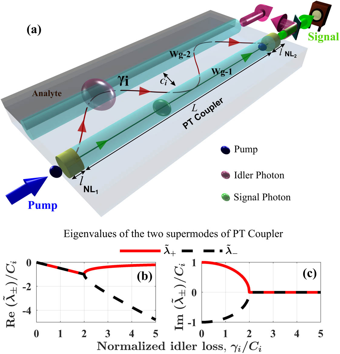
(a) Sketch of hybrid nonlinear interferometer incorporating a PT coupler for sensing of analyte-induced absorption (γi) in waveguide Wg-2. Dependence of (b) real and (c) imaginary parts of normalized eigenvalues, λ˜±/Ci, which account for the loss and wavenumber respectively, on the normalized loss γi/Ci for the two idler supermodes of symmetric PT coupler composed of Wg-1 and Wg-2.

Figure 1.(a) Sketch of hybrid nonlinear interferometer incorporating a PT coupler for sensing of analyte-induced absorption ( $γ_{i}$ ) in waveguide Wg-2. Dependence of (b) real and (c) imaginary parts of normalized eigenvalues, ${\tilde{λ}}_{\pm} / C_{i}$ , which account for the loss and wavenumber respectively, on the normalized loss $γ_{i} / C_{i}$ for the two idler supermodes of symmetric PT coupler composed of Wg-1 and Wg-2.

2. NONLINEAR INTERFEROMETER INTEGRATING A PT-SYMMETRIC COUPLER

A. Design of Interferometer

We consider an integrated nonlinear interferometer based on waveguides (Wgs) as shown in Fig. 1(a). It consists of a pair of evanescently coupled Wgs where Wg-2 interacts with an analyte that can introduce losses to form a passive PT coupler. Two short sections of Wg-1, shown in yellow and denoted by ${NL}_{1}$ and ${NL}_{2}$ , possess a quadratic nonlinear susceptibility and function as SPDC sources of signal–idler photon pairs when pumped by a continuous wave laser; here shown as the pump. On the other hand, the section of Wg-1 between ${NL}_{1}$ and ${NL}_{2}$ acts as a purely linear element. In practice, such a configuration of linear and nonlinear elements can be easily realized within the same physical Wg made out of quadratic nonlinear materials by engineering the spatial distribution of their effective nonlinearity through quasi-phase matching (QPM) [35]. For instance, sections ${NL}_{1}$ and ${NL}_{2}$ could be periodically poled to modulate their nonlinearity at period $Λ$ , while the portion between these could be left unpoled. Assisted by the additional grating vector, $K = 2 π / Λ$ , arising from the QPM poling, the SPDC process can occur efficiently in the two poled sections while the central section merely acts as a dispersive linear element.

Whereas a simple device geometry employing two spatially separated sources of photon pairs in a single Wg (here Wg-1) can already function as a nonlinear interferometer [20], the key suggestion of this work is to introduce a second linear waveguide (Wg-2) adjacent to Wg-1. We show that this enriches the response of the nonlinear interferometer by making use of the exceptional dispersive properties of the resulting PT coupler.

Throughout this paper, we consider the operation of SPDC in the nonlinear sections in the nondegenerate wavelength regime such that the idler photon wavelength is $λ_{i} > 2 μm$ while the pump and signal wavelengths lie in the $λ_{p, s} < 1 μm$ range [10,36,37]. Although the exact wavelengths of operation can be suitably chosen as needed by the application, the ranges we indicate here are meant to convey the intended utility of the scheme in facilitating spectroscopic applications in the technologically important mid-infrared spectral range with detection and excitation wavelengths being in the visible or near-infrared range.

A salient feature of our proposed design is that the separation distance between Wg-1 and Wg-2 can be suitably chosen so that the longer wavelength idler photon generated in ${NL}_{1}$ can tunnel to Wg-2 with coupling rate $C_{i}$ and evanescently interact with the analyte deposited in its vicinity. At the same time, the shorter wavelength pump and signal photons remain confined to Wg-1 and do not interact with the analyte. However, the idler photon can tunnel back into Wg-1 ensuring that the biphoton amplitude emanating from ${NL}_{1}$ can interfere with that from ${NL}_{2}$ . Due to the nonlocal nature of this quantum interference, the effective absorption strength in Wg-2, denoted as $γ_{i}$ , can be determined by counting just the signal photons at the output of Wg-1. Note that neither the pump nor the signal photons ever propagate through Wg-2 in this scheme.

B. PT Coupler

Before we discuss the generation and evolution of photon pairs in the complete interferometer structure shown in Fig. 1(a), we provide a brief description of the evolution of classical optical fields within the linear PT coupler between the photon-pair sources. Since the pump and signal fields remain confined to Wg-1, the evolution of their field amplitudes, $a_{p, s} (z)$ , is described by $\partial a_{p, s} (z) / \partial z = - i β_{p, s} \cdot a_{p, s} (z)$ with $β_{p, s}$ being their respective propagation constants. On the other hand, the idler field can couple to Wg-2 and, therefore, its field amplitude is described by a two-dimensional vector, $A_{i} (z) = {[\begin{matrix} a_{i}^{(1)} (z) & a_{i}^{(2)} (z) \end{matrix}]}^{T}$ whose evolution is given by $\frac{\partial A_{i} (z)}{\partial z} = M_{i} A_{i} (z),$ (1)with $M_{i} = [\begin{matrix} - i ({\bar{β}}_{i} + Δ β_{i}) & - i C_{i} \\ - i C_{i} & - i ({\bar{β}}_{i} - Δ β_{i}) - γ_{i} \end{matrix}] .$ (2)

Here, ${\bar{β}}_{i} \equiv (β_{i}^{(1)} + β_{i}^{(2)}) / 2$ and $Δ β_{i} \equiv (β_{i}^{(1)} - β_{i}^{(2)}) / 2$ are defined in terms of the idler propagation constants $β_{i}^{(1, 2)}$ of the two uncoupled Wgs. The loss coefficient $γ_{i}$ is responsible for idler loss in the coupler and is present exclusively in Wg-2. Finally, $C_{i}$ denotes the coupling constant between Wg-1 and Wg-2. Solutions of Eq. (1) can be obtained analytically by making use of the eigenvalues $λ_{\pm} = - i {\bar{β}}_{i} + {\tilde{λ}}_{\pm}$ and corresponding eigenvectors $V_{\pm}$ of the coupler propagation matrix $M_{i}$ , which are ${\tilde{λ}}_{\pm} = \frac{\pm ξ_{i} - γ_{i}}{2}, V_{+} = {[\begin{matrix} γ_{i} + ξ_{i} - 2 i Δ β_{i} & - 2 i C_{i} \end{matrix}]}^{T}, V_{-} = {[\begin{matrix} 2 i C_{i} & γ_{i} + ξ_{i} - 2 i Δ β_{i} \end{matrix}]}^{T},$ (3)where $ξ_{i} = \sqrt{{(γ_{i} - 2 i Δ β_{i})}^{2} - {(2 C_{i})}^{2}}$ and $A_{i} (z) = α_{+} e^{λ_{+} z} V_{+} + α_{-} e^{λ_{-} z} V_{-} .$ (4)

The coefficients $α_{\pm}$ are determined by the input fields to the coupler. The eigenvectors $V_{\pm}$ describe the two supermodes of the coupler in terms of the individual modes of the two Wgs. The corresponding eigenvalues define their complex propagation constants, which depend on the idler loss magnitude $γ_{i}$ in a nontrivial manner as is evident from the expression for ${\tilde{λ}}_{\pm}$ .

We display the characteristic dependence of $Re ({\tilde{λ}}_{\pm})$ and $Im ({\tilde{λ}}_{\pm})$ , which describe the loss and wavenumber of the supermodes for a symmetric coupler ( $Δ β_{i} = 0$ ), in Figs. 1(b) and 1(c). The effect of PT symmetry breaking [22] occurs at $γ_{i} / C_{i} = 2$ . For idler losses below this threshold value, the two supermodes of the PT coupler have the same effective losses equal to $γ_{i} / 2$ [see Fig. 1(b)]. This symmetry between supermodes $V_{\pm}$ is due to the nature of their composition in terms of individual modes of the two Wgs below the threshold loss, with $‖ V_{\pm}^{(1)} ‖ = ‖ V_{\pm}^{(2)} ‖$ . Above the PT symmetry breaking point, $V_{+}$ starts to localize in Wg-1 with $‖ V_{+}^{(1)} ‖ > ‖ V_{+}^{(2)} ‖$ while $V_{-}$ localizes in Wg-2. Consequently, the loss coefficient for the $V_{+}$ supermode decreases with increasing $γ_{i}$ , while the opposite is true for the $V_{-}$ supermode. As we demonstrate in the following, this has a characteristically defining effect on the behavior of the proposed nonlinear interferometer. Another important feature to note here is the dependence of $Im ({\tilde{λ}}_{\pm})$ on $γ_{i}$ which is shown in Fig. 1(c). Both supermodes of the coupler have loss-dependent wavenumbers only below the PT symmetry breaking point. In the broken symmetry regime, they become independent of $γ_{i}$ .

3. METHODS AND RESULTS

After reviewing the linear properties of the PT coupler, we now show its profound influence on photon-pair generation in a nonlinear interferometer and discuss applications of the ensuing interference phenomena for quantum sensing. To mathematically describe the behavior of the proposed nonlinear interferometer, we draw upon the theoretical formulation developed in Refs. [38,39] for describing the process of photon-pair generation through SPDC and its propagation in lossy media. We simplify the analysis of pair generation in the nonlinear sections ${NL}_{1}$ and ${NL}_{2}$ by assuming that their lengths $l$ are much smaller than the coupling length for the idler photon ( $l ≪ π / 2 C_{i}$ ). Hence, in the following we neglect the effect of coupling between Wg-1 and Wg-2 when describing the evolution of signal–idler biphoton amplitudes in the nonlinear sections. We must note here that our assumption about small nonlinear section lengths is not fundamental to the effects we demonstrate in this work. In fact, for practical implementation, one can choose a coupler design where Wg-1 bends away at the beginning and end of the structure to decouple the waveguides and nonlinear sections of arbitrary lengths can then be placed in these uncoupled regions in Wg-1. In such a design, pair generation in the first and second nonlinear sections will be unaffected by the loss in the coupler section.

A. Biphoton State Amplitude Evolution

We calculate biphoton amplitudes for the quantum state in the Wg number basis. This is primarily because this basis provides a clear understanding of the spatial dynamics of the generation and propagation of the photon pairs. The state is described by three probability amplitudes [38] corresponding to the three possible localizations of the signal and idler photons: $ϕ_{11}$ : signal–idler pair is jointly present in Wg-1, $ϕ_{12}$ : signal is present in Wg-1 while idler is in Wg-2, $ϕ_{12}^{(s)}$ : signal is in Wg-1 and idler photon is absorbed in Wg-2.

In this section, we first focus on the evolution of the pair amplitudes $ϕ = {[\begin{matrix} ϕ_{11} & ϕ_{12} \end{matrix}]}^{T}$ ; the evolution of $ϕ_{12}^{(s)}$ is discussed in the subsequent section. The Schrödinger-type equations for evolution of $ϕ_{11} (z)$ and $ϕ_{12} (z)$ in each of the nonlinear sections are given by [40] $\frac{\partial ϕ_{1, n_{i}} (z)}{\partial z} = - i (β_{s} + β_{i}^{(n_{i})}) ϕ_{1, n_{i}} (z) + δ_{1, n_{i}} A_{p} (z),$ (5)where the subscript $n_{i}$ refers to the number of the Wg, 1 or 2, in which the idler photon could be present while its partner signal photon is confined to Wg-1, and the Kronecker delta function $δ_{1, n_{i}}$ represents the fact that pair generation can occur only in Wg-1 where the classical pump field given by $A_{p} (z) = A_{p} (0) \times \cos (K z) \times \exp (- i β_{p} z)$ is present. Here, $A_{p} (0)$ subsumes the strength of the quadratic nonlinearity and the factor $\cos (K z)$ represents the dominant spatial modulation of the nonlinearity that realizes QPM in the two nonlinear sections with $K = 2 π / Λ$ . Poling period $Λ$ is chosen such that ${\bar{β}}_{p} - {\bar{β}}_{s} - {\bar{β}}_{i}^{(1)} - K = 0$ for a specific set of pump, signal, and idler modes. By neglecting the coupling between the two waveguides in Eq. (5), we implicitly also have neglected the effects of idler loss in Wg-2 on the biphoton evolution in the nonlinear sections. The solution of Eq. (5) for the first nonlinear section ${NL}_{1}$ with $0 \leq z \leq l$ gives the photon-pair amplitude originating from the first source. At $z = l$ this is $ϕ (l) = {[\begin{matrix} 1 & 0 \end{matrix}]}^{T} ϕ_{0} (l)$ (6)with $ϕ_{0} (l) = [A_{p} (0) l / 2] \cdot e^{- i (β_{s} + β_{i}^{(1)} + \frac{Δ β_{NL}}{2}) l} sinc (\frac{Δ β_{NL} l}{2}),$ (7)where $Δ β_{NL} = β_{p} - β_{s} - β_{i}^{(1)} - K$ denotes the phase mismatch for SPDC in ${NL}_{1}$ and ${NL}_{2}$ .

Within the PT coupler section of length $L$ , the evolution of amplitude $ϕ (z) = {[\begin{matrix} ϕ_{11} (z) & ϕ_{12} (z) \end{matrix}]}^{T}$ is governed by $\frac{\partial ϕ (z)}{\partial z} = (- i β_{s} 1 + M_{i}) ϕ (z),$ (8)where we have used the propagation matrix $M_{i}$ from Eq. (1). We propagate the photon-pair amplitudes generated in ${NL}_{1}$ through the coupler section of the interferometer with $l \leq z \leq l + L$ by solving Eq. (8) making use of the eigenvalues and eigenvectors of matrix $(- i β_{s} 1 + M_{i})$ . At $z = l + L$ , this results in $ϕ (l + L) = e^{- i (β_{s} + {\bar{β}}_{i}) L} e^{- γ_{i} L / 2} \times [\begin{matrix} \cosh^{2} Θ e^{ξ_{i} L / 2} - \sinh^{2} Θ e^{- ξ_{i} L / 2} \\ i \sinh Θ \cosh Θ (e^{- ξ_{i} L / 2} - e^{ξ_{i} L / 2}) \end{matrix}] ϕ_{0} (l),$ (9)where $\sinh Θ \equiv (2 C_{i}) / \sqrt{{(γ_{i} + ξ_{i} - 2 i Δ β_{i})}^{2} - {(2 C_{i})}^{2}}$ and $\cosh^{2} Θ - \sinh^{2} Θ = 1$ (see Appendix A for details of derivation). Finally, to obtain the complete biphoton state amplitude at the end of the interferometer, $z = 2 l + L$ , we superpose the photon-pair amplitudes in Eq. (9) with the pair generation amplitude arising from the second source, ${NL}_{2}$ . This results in the amplitude $ϕ (2 l + L) = [\begin{matrix} e^{- i β_{i}^{(1)} l} & 0 \\ 0 & e^{- i β_{i}^{(2)} l} \end{matrix}] e^{- i β_{s} l} ϕ (l + L) + [\begin{matrix} 1 \\ 0 \end{matrix}] ϕ_{0} e^{- i β_{p} (l + L)},$ (10)where we note that the second nonlinear source can contribute only to $ϕ_{11}$ since both photons are generated in and remain confined to Wg-1 due to this source.

B. Measurable Signal Photon Intensity

Quantum spectroscopy based on nonlinear interference and induced coherence requires only detection of the signal photon intensity. In the implementation discussed here, depicted in Fig. 1(a), the intensity measurement is performed only on the signal mode in Wg-1, as the signal photon generated in either source will not couple to Wg-2. The detection of a signal photon in Wg-1 could result from one of three possibilities for the state of the idler photon shown schematically in Fig. 2(a), corresponding to the three probability amplitudes $ϕ_{11}$ , $ϕ_{12}$ , and $ϕ_{12}^{(s)}$ . These possibilities are distinguishable, and hence the total signal intensity is a sum of the intensities of the three contributions as $I_{1}^{s} = I_{11} + I_{12} + I_{12}^{(s)} .$ (11)

Figure 2.(a) Top panel shows waveguides in which signal and idler photons are present for the biphoton ( $I_{11}$ & $I_{12}$ ) and single photon $I_{12}^{(s)}$ intensity contributions (see text for their description). (b) For lossless PT coupler, biphoton amplitudes from sources ${NL}_{1}$ and ${NL}_{2}$ interfere destructively. (c) At the critical loss, $γ_{i} = γ_{cr}$ , pair generation in ${NL}_{1}$ and ${NL}_{2}$ becomes totally distinguishable and their amplitudes add up incoherently. (d) In the broken PT regime, the nonlinear interferometer exhibits increased indistinguishability and coherence between pair generation amplitudes from the two sources. In (b)–(d), a special coupler design with $C_{i} L = π$ is considered.

Here, the intensity contributions stemming from the two-photon amplitudes can be directly calculated from Eq. (10) as $I_{11} (z) = | ϕ_{11} (z {) |}^{2}$ , $I_{12} (z) = | ϕ_{12} (z {) |}^{2}$ . Next, we derive the $I_{12}^{(s)}$ contribution to the signal intensity. The probability amplitude for detecting the signal photon at position $z$ with its partner idler photon being absorbed at position $z^{'}$ is given by $ϕ_{12}^{(s)} (z, z^{'})$ . Following Ref. [38], its evolution is given by $\frac{\partial ϕ_{12}^{(s)} (z, z^{'})}{\partial z} = {\begin{cases} - i β_{s} ϕ_{12}^{(s)} (z, z^{'}) & for z^{'} \leq z \\ 0 & otherwise \end{cases},$ (12)with the initial condition $ϕ_{12}^{(s)} (z^{'}, z^{'}) = - i \sqrt{2 γ_{i}} ϕ_{12} (z^{'})$ . The signal intensity $I_{12}^{(s)} (z)$ is accumulated over the length of the coupler from the absorbed idler amplitudes $ϕ_{12}^{(s)} (z, z^{'})$ and is equal to $I_{12}^{(s)} (z) = \int_{l}^{z} {| ϕ_{12}^{(s)} (z, z^{'}) |}^{2} d z^{'} = 2 γ_{i} \int_{l}^{z} {| ϕ_{12} (z^{'}) |}^{2} d z^{'}, for z > l,$ (13)with $I_{12}^{(s)} (l) = 0$ . The second nonlinear source does not contribute to this amplitude, since it is assumed to be lossless and not coupled to Wg-2.

Overall, we find that the second nonlinear section can only affect $I_{11}$ . Only the first source ${NL}_{1}$ placed before the coupler can contribute to all three intensities $I_{11}$ , $I_{12}$ , and $I_{12}^{(s)}$ . Hence, the two sources only interfere, if ${NL}_{1}$ contributed to $I_{11}$ at the end of the structure, since both sources are indistinguishable in this intensity component. This means that induced coherence between the sources can only appear if there is a nonzero probability for the idler photon from ${NL}_{1}$ to be located in Wg-1 in the region ${NL}_{2}$ . The dynamics of induced coherence is thus dependent on the state of the idler photon generated from ${NL}_{1}$ , which itself is controlled by the properties of the coupler, i.e., its coupling strength, length, and the loss in Wg-2.

C. Constructive and Destructive Photon Interference and Its Dependence on Idler Loss

To fully understand the dependence of induced coherence between the sources and the resulting interference in the signal intensity on the idler loss, we explicitly calculate the intensity stemming from the case where both photons are in Wg-1 using Eqs. (10) and (9), as this is the only contribution to the signal intensity that can show interference. It is $I_{11} (2 l + L) = {1 + {| V_{γ_{i}} |}^{2} + 2 Re [V_{γ_{i}} \times e^{i (Δ β_{NL} + K) (L + l)}]} {| ϕ_{0} |}^{2},$ (14)with $V_{γ_{i}} = e^{i Δ β_{i} L - γ_{i} L / 2} [\cosh \frac{ξ_{i} L}{2} + (1 + 2 \sinh^{2} Θ) \sinh \frac{ξ_{i} L}{2}] .$ (15)

In $I_{11}$ , coherence between pair generation amplitudes from the two sources is clearly manifested in the last term of Eq. (14), where the visibility of the resulting interference fringes as a function of $Δ β_{NL}$ is determined by parameter $V_{γ_{i}}$ . The other contributions to the signal intensity can only result from photon-pair generation in the first nonlinear section ${NL}_{1}$ , and the explicit expressions for intensities $I_{12} (2 l + L)$ and $I_{12}^{(s)} (2 l + L)$ do not show any signature of interference like $I_{11} (2 l + L)$ (see Appendix B). As such, the magnitude of $| V_{γ_{i}} |$ could be regarded as the measure of the indistinguishability of the two photon-pair sources in the interferometer enabling interference in the resulting signal intensity.

We see from Eq. (14) that whether the interference is constructive or destructive depends on the additional phase acquired by the idler photon as it propagates through the PT coupler. This is encapsulated in $V_{γ_{i}}$ , which is defined through the coupler asymmetry, the coupling strength, the length of the coupler, and the idler loss.

For a symmetric coupler with equal real parts of the idler propagation constants in both waveguides, $Δ β_{i} = 0$ , the expression in Eq. (15) simplifies to $V_{γ_{i}} = e^{- \frac{γ_{i} L}{2}} (\cos \frac{σ_{i} L}{2} + \frac{γ_{i}}{σ_{i}} \sin \frac{σ_{i} L}{2}) with σ_{i} = \sqrt{{(2 C_{i})}^{2} - γ_{i}^{2}}$ (16)below the PT threshold loss, $γ_{i} \leq 2 C_{i}$ . Above PT threshold loss $γ_{i} > 2 C_{i}$ , $V_{γ_{i}}$ can be similarly shown to be $V_{γ_{i}} = e^{- \frac{γ_{i} L}{2}} (\cosh \frac{η_{i} L}{2} + \frac{γ_{i}}{η_{i}} \sinh \frac{η_{i} L}{2}) with η_{i} = \sqrt{γ_{i}^{2} - {(2 C_{i})}^{2}} .$ (17)

We note from Eqs. (16) and (17) that $V_{γ_{i}}$ is a real function and depends on idler loss $γ_{i}$ . Further, only constructive interference is possible in the PT-broken regime, since $V_{γ_{i}} > 0$ according to Eq. (17). Importantly, the sign of $V_{γ_{i}}$ is unrestricted in the PT-symmetric regime. The transition between constructive and destructive interference can therefore occur at a critical idler loss $γ_{cr}$ , when $V_{γ_{cr}} = 0 .$ (18)

These features can be employed to tailor the interferometer response to loss variations as we discuss below.

D. Evolution of Photon Intensities

We show the characteristic evolution of the different intensity contributions along the interferometer in Figs. 2(b)–2(d) for three different values of loss in Wg-2. We consider the case of phase-matched SPDC with $Δ β_{NL} = 0$ and a symmetric PT coupler where $Δ β_{i} = 0$ . The relative phase between pair amplitudes from the two sources stems from the constant phase factor $K (L + l)$ and the loss-dependent phase of $V_{γ_{i}}$ . For simplicity, here we assume that the QPM grating vector is such that $K (L + l) = 2 n π$ with $n \in N$ , resulting in constructive biphoton interference if no coupling was present between the two Wgs. However, since coupling is present, the phase of $V_{γ_{i}}$ additionally modifies the interference. To maximize the photon-pair interference in the second nonlinear section, we choose the length of the PT coupler equal to twice the coupling length in absence of loss, corresponding to $C_{i} L = π$ . The nonlinear section length is taken to be $C_{i} l = 0.05$ , much less than the coupling length. In practice, nonlinear section length $l$ can be always suitably chosen to ensure that $K (L + l) = 2 n π$ if the coupler length $L$ has to be kept constant. In the following numerical simulations, we keep the normalized value of the coupling constant fixed as $C_{i} = 1$ with no loss of generality. Other parameters such as lengths, propagation constants, and losses are assumed to be appropriately scaled by $C_{i}$ and rendered dimensionless. As an example for a coupler with the physical coupling of $C_{i} = 0.5 {cm}^{- 1}$ [40], the normalized length of $L = π$ corresponds to a physical length $L = π / C_{i} = 2 π cm$ and the normalized idler loss of $γ_{i} = 2$ for PT threshold loss corresponds to an actual loss of $γ_{i} = 2 C_{i} = 1 {cm}^{- 1}$ .

We present in Fig. 2(b) the Hermitian case in which the PT coupler is lossless with $γ_{i} = 0$ . In this case, the idler photon of the pair generated in ${NL}_{1}$ completely couples to Wg-2 and back such that $| ϕ_{11} (l + L) | = | ϕ_{11} (l) |$ while $I_{12} (l + L) = 0$ . The photon-pair amplitude generated in ${NL}_{2}$ is coherently added to the amplitude stemming from ${NL}_{1}$ , which in the considered case leads to complete destructive interference and a signal intensity of zero at the end of the interferometer. This is the manifestation of the fact that in this case the contributions of the two nonlinear sections to the photon-pair amplitude are indistinguishable, enabling interference. Indeed, for the considered parameters according to Eq. (16) the visibility parameter is $V_{γ_{i}} = \cos (C_{i} L)$ , leading to $V_{γ_{i}} = - 1$ for the chosen coupler length, such that the final biphoton intensity $I_{11}$ becomes zero. Since no loss is present in Wg-2, the signal photon amplitude associated with the absorbed idler photon is also zero in this case (see $I_{12}^{(s)}$ ) and thus, the total final signal intensity $I_{1}^{s}$ vanishes. The intensity values plotted in these figures are normalized by the maximum possible signal intensity which, as we discuss later, is attained for infinitely large idler loss in the considered coupler design.

Introducing loss in Wg-2 for the idler photon changes the response of the interferometer. We show this in Fig. 2(c) for a loss $γ_{i} = γ_{cr} = 1.35$ according to Eq. (18), which we refer to as the critical loss. At $γ_{cr}$ , at the end of the PT coupler, the idler photon of a pair generated in ${NL}_{1}$ is either present in Wg-2 or is absorbed in Wg-2 during propagation in the coupler, such that $I_{11} (l + L) = 0$ . Therefore, in this case, no interference takes place between the two sources, because they are completely distinguishable and $I_{11} (2 l + L)$ only contains contributions from the second source ${NL}_{2}$ . Consequently, the final output signal intensity $I_{1}^{s} (2 l + L)$ from the interferometer results from a completely incoherent addition of pair amplitudes originating from the two sources.

We note that in standard implementations of quantum nonlinear interferometers [6], biphoton amplitudes from individual sources approach complete distinguishability, leading to their fully incoherent addition and the absence of interference, only at infinitely high losses. Due to the interplay of coupling and loss in our structure, complete distinguishability can be reached for the finite loss $γ_{cr}$ . As we show in the following, the value of $γ_{cr}$ can be controlled by appropriately choosing the coupling constant and length of the PT coupler. We also find that even several such critical loss values can exist for a particular structure, where for a fixed coupling strength the coupler length has to be made longer to increase the number of critical points corresponding to complete distinguishability (see Appendix B).

The behavior of the interferometer is quite different for losses above the PT symmetry breaking threshold $γ_{th} = 2 C_{i}$ , since the points of critical loss exist only in the PT-symmetric regime as discussed in Section 3.C. This aspect is reflected in Fig. 2(d), where we plot the various intensity contributions at a loss magnitude of $γ_{i} = 5$ . Here, the final signal intensity $I_{1}^{s} (2 l + L)$ as well as $I_{11} (2 l + L)$ is larger compared to Fig. 2(c) despite stronger loss. This apparently counter-intuitive result can be explained by considering the propagation dynamics of the idler photon in the PT coupler for different losses. The nature of the two supermodes $V_{\pm}$ and their corresponding eigenvalues dictate the idler photon dynamics as expressed by Eq. (4). As discussed before, these eigenmodes of the PT coupler remain symmetric in the two Wgs below $γ_{th}$ and exhibit equal losses as is shown in Fig. 1(b). For losses above $γ_{th}$ , this symmetry is broken and the two Wgs start to effectively decouple from each other. The $V_{+}$ eigenmode, with its corresponding eigenvalue shown by the red solid curve in Figs. 1(b) and 1(c) tends to be localized in the lossless Wg-1, while the other eigenmode localizes in the lossy Wg-2. As a result, the $V_{+}$ mode experiences progressively lower effective losses while the $V_{-}$ mode becomes increasing lossy in the broken PT regime. Since the first source ${NL}_{1}$ is positioned in Wg-1 in the interferometer, its biphoton amplitude favorably excites the $V_{+}$ idler supermode in the broken PT regime and hence, the idler may experience lower effective losses for $γ > γ_{th}$ . As this supermode features a high probability for the idler photon to be localized in Wg-1, this means that also $I_{11} (l + L)$ is increased for $γ > γ_{th}$ , which can interfere with the contribution from ${NL}_{2}$ . Hence, the indistinguishability of pair generation between the two sources is improved as the idler loss strength increases in Wg-2 in the broken PT regime.

E. Signal Fringes and Sharp Transition at Critical Loss

After discussing the signal intensity evolution within the structure for several specific values of idler loss and a fixed phase mismatch, we now explicitly demonstrate the sharp change in the behavior of the interferometer around the critical loss magnitude for a varying mismatch $Δ β_{NL}$ . In experimental realizations, this mismatch usually corresponds to the wavelength of the detected signal mode for a fixed pump wavelength.

We show in Fig. 3(a) the dependence of the total signal intensity $I_{1}^{s}$ on the idler loss strength $γ_{i}$ and the phase mismatch parameter $Δ β_{NL}$ . We clearly observe the fringes as a function of $Δ β_{NL}$ . The phase mismatch is normalized by $C_{i}$ , so the period of intensity fringes given by $Δ β_{NL} = 2$ here, corresponds to an actual phase shift of $Δ β_{NL} \cdot L = 2 π$ . For zero loss, the visibility of interference is perfect, being equal to unity, and the interference maxima appear for specific $Δ β_{NL}$ . As $γ_{i}$ increases, the visibility is reduced, and it completely vanishes exactly at the critical loss $γ_{cr} = 1.35$ .

Figure 3.Normalized total signal intensity $I_{1}^{s}$ versus the idler absorption strength ( $γ_{i}$ ) and phase mismatch parameter ( $Δ β_{NL}$ ). (a) In a symmetric coupler, $β_{i}^{(2)} = β_{i}^{(1)}$ , the signal intensity fringe position exhibits a sharp shift by half a period at the critical loss $γ_{i} = γ_{cr}$ . (b) For the asymmetric coupler with $Δ β_{i} = 0.2$ , the signal fringe position shifts gradually with the absorption strength. For all the plots, $C_{i} L = π$ and $C_{i} = 1$ .

Strikingly, the signal intensity fringe exhibits a sharp shift by half a period as the idler loss strength changes across this critical loss magnitude. This is illustrated by the blue dashed line overlaid on the signal intensity contour plot that tracks the position of the central intensity maximum. We also see that such behavior does not occur with increasing idler losses beyond the PT threshold loss $γ_{th} = 2$ . In fact, the signal intensity fringe acquires a specific position in $Δ β_{NL}$ and its visibility improves with increasing idler loss.

This behavior of the signal intensity fringes and the associated visibility with increasing idler loss are due to the interference of photon-pair amplitudes from the two sources. For zero loss, $γ_{i} = 0$ , with the chosen PT coupler parameters, $C_{i} L = π$ , the idler photon probability amplitude from the first source, tunnels to Wg-2 and comes back completely to Wg-1 at the second nonlinear source. This leads to perfect indistinguishability between the sources and the resulting signal interference fringe shows maximum visibility. In contrast, at the critical idler loss, $γ_{i} = γ_{cr}$ , the two sources are completely distinguishable since the idler photon, if generated in the first source, is either present in the Wg-2 at the end of the interferometer or is absorbed during propagation in the coupler. This leads to the vanishing of signal interference visibility. Further increasing the idler loss reduces the effective coupling between waveguides and increases the probability that the idler photon amplitude from the first source remains in Wg-1 when it reaches the end of the coupler section of the interferometer. This leads to the recovery of the interference visibility since the sources become partially indistinguishable again.

We have, thus far, only visualized the case of the symmetric coupler where the two Wgs have equal propagation constants for the idler mode, i.e., $β_{i}^{(2)} = β_{i}^{(1)}$ and thus $Δ β_{i} = 0$ . We now analyze the effect of breaking this symmetry when $Δ β_{i} \neq 0$ . The resulting signal intensity behavior is displayed in Fig. 3(b) for a detuning magnitude of $Δ β_{i} = 0.2$ . Unlike the PT-symmetric case, the interferometer employing the asymmetric coupler shows a gradual shift in the position of the signal intensity fringe with a change in the idler loss strength. Also, the visibility of the interference does not reduce to zero for any specific loss value.

F. Sensing of Idler Losses

Based on the nontrivial dependence of the signal intensity on the idler loss, next we suggest a specific sensing application of our scheme. We have shown the dependence of the interference fringes on the loss in Fig. 3(a), and we explicitly show the associated variation of their visibility in Fig. 4(a) with the red curve. Here, the visibility $V$ of the signal interference fringe for loss $γ_{i}$ is calculated as $V = [\max_{Δ β_{NL}} (I_{1}^{s}) - \min_{Δ β_{NL}} (I_{1}^{s})] / [\max_{Δ β_{NL}} (I_{1}^{s}) + \min_{Δ β_{NL}} (I_{1}^{s})]$ , where $I_{1}^{s} (L + 2 l)$ is the signal intensity as a function of the phase mismatch $Δ β_{NL}$ at constant loss magnitude. We note that $V$ is different from the visibility parameter $V_{γ_{i}}$ discussed before for the $I_{11}$ intensity due to the contributions of $I_{12}$ and $I_{12}^{(s)}$ to the total signal intensity.

Figure 4.(a) Visibility $V$ of the interference in the signal intensity at the end of the nonlinear interferometer containing the PT coupler versus the idler loss for different coupler lengths. (b) Corresponding normalized total signal intensity at $Δ β_{NL} = 0$ . The dots denote the boundaries of regions where the visibility is below 0.05 and the intensity is close to 0.5. (c) Sensitivity $| \frac{d V}{d γ_{i}} |$ for visibility and (d) sensitivity $| \frac{d I_{1}^{s}}{d γ_{i}} |$ for narrowband signal intensity measurements.

In Fig. 4(a), we mark a region in gray where the visibility $V$ is below 0.05. This value can serve as a specific threshold magnitude of visibility below which interference fringes cannot be detected reliably. We have highlighted the corresponding two points on the red curve between which the visibility is below this threshold value. The critical loss $γ_{cr}$ , for which the visibility vanishes completely, lies between these two points. In Fig. 4(b) we show the corresponding signal intensity $I_{1}^{s} (Δ β_{NL} = 0)$ for the phase-matched case along with the two threshold visibility points. In the intermediate region between these points, we have $I_{1}^{s} \approx 0.5 \times I_{1}^{s} (γ_{i} \to \infty)$ [see Fig. 4(b)], signifying that the two sources of photon pairs are almost distinguishable. Hence, no notable interference pattern in the signal intensity can be observed.

The range of loss magnitudes where the two photon-pair sources are nearly completely distinguishable and the visibility is very close to zero can be controlled by adapting the design parameters of the nonlinear interferometer. We show this by considering designs with couplers of lengths $L = 2 π$ and $3 π$ , shown in Figs. 4(a) and 4(b) with the blue and black curves, respectively. The visibility plots clearly show that a larger loss region with visibilities below 0.05 can be realized for longer coupler lengths with several critical loss points lying within this region. It is important to realize that all such critical points lie below the PT-symmetry-breaking threshold $γ_{th} = 2$ . Furthermore, for loss magnitudes within this region, the signal intensity stays almost constant, regardless of the precise value of the loss (see Appendix B). The variation of the signal intensity with changing idler loss measured through its slope $| d I_{1}^{s} / d γ_{i} |$ can be regarded as a figure-of-merit to gauge the sensitivity of the measurement scheme for sensing idler loss when measurements are made at a given signal wavelength. Alternatively, for broadband signal intensity fringe measurements sensitivity can be defined through the fringe visibility in terms of its slope $| d V / d γ_{i} |$ for various idler losses. We show the variation of these sensitivity parameters in Figs. 4(c) and 4(d). Both of these plots show similar overall behavior. The cases with $L = 2 π$ and $L = 3 π$ are characteristically different from $L = π$ in that the sensitivities reduce to zero at certain idler losses below the PT threshold loss unlike the $L = π$ case and become nonzero again for increasing losses. In fact, there is a range of loss within which both $| d V / d γ_{i} |$ and $| d I_{1}^{s} / d γ_{i} |$ have very small magnitudes.

The peculiar features discussed above could be applicable to sensing scenarios that require determination of whether the concentration of the analyte responsible for the loss is within a specific target range. Importantly, the boundaries of the range with approximately constant signal intensity can be fixed by appropriately choosing the length and coupling strength of the PT coupler. For such target loss-range sensing it is important that the signal intensity changes appreciably with change in loss when the background loss goes outside the specified range. For the two design cases shown in Figs. 4(a) and 4(b) with $L = 2 π$ and $3 π$ , the slope of signal intensity is larger than with $L = π$ for small losses. At the same time, the design with $L = 2 π$ shows a larger variation of signal intensity and a higher fringe visibility for losses $γ_{i} > 2$ compared to the $L = 3 π$ case. Hence, it is important to choose an appropriate length of the coupler that can provide sufficiently large sensitivities outside of the target range. We find that for longer couplers the sensitivity at larger losses is reduced, while at very small losses the sensitivity is increased, as shown by the plots in Figs. 4(c) and 4(d). Importantly, our suggested device can be preferably used to sense very high absorption. Here, contrary to standard nonlinear interferometers, the visibility of interference is revived and increasing for larger losses, as shown by Fig. 4(a), which renders their detection easier.

It is instructive to compare the proposed nonlinear interferometric sensing scheme with the conventional linear absorption sensing based on a PT coupler, in which laser light at the idler wavelength is transmitted through the coupler and detected at its end. As was shown in Ref. [22], the transmitted intensity in such a scheme shows a nontrivial dependence on the absorption loss such that it first decreases with increasing losses up to a certain loss value and then starts to increase with increasing losses. In our work, we employ the unconventional transmission property of the PT coupler for the idler photon. However, the most important difference of the presented scheme is that we utilize the spectral correlation of the signal–idler pairs generated through SPDC in the nonlinear sections of the interferometer to effectively transfer the information about the losses at the longer idler wavelength to the short-wavelength signal-photon spectrum. This makes it possible to employ highly sensitive and low-noise detectors to measure the signal intensity and infer the losses at the idler wavelength.

G. Broadband Absorption Spectroscopy

Spectroscopic applications employing nonlinear interferometers typically aim to achieve operation in a broad spectral range such that the frequency-dependent absorption profile of an analyte can be measured around the idler photon frequency by performing detection at the corresponding frequencies of the signal photon. Such operation is essentially achieved by employing broadband SPDC in the interferometer where two short nonlinear sources of photon pairs are pumped by a continuous-wave pump laser at a fixed frequency. We now perform a similar frequency-dependent loss analysis for the interferometric scheme that we propose in this work.

To illustrate the spectral response, we start by considering the frequency dependence of the phase mismatch parameter $Δ β_{NL}$ due to the dispersion of signal and idler modes. Under a first-order approximation, the propagation constants of the signal and idler modes can be described as $β_{s, i}^{(1)} ({\bar{ω}}_{s, i} + Δ ω_{s, i}) = β_{s, i}^{(1)} ({\bar{ω}}_{s, i}) + {(1 / v_{g})}_{s, i} \times (Δ ω_{s, i})$ , where ${\bar{ω}}_{s, i}$ are the respective central frequencies and $v_{g}$ denotes the group velocity at these frequencies. Assuming a continuous wave pump at frequency $ω_{p} = {\bar{ω}}_{s} + {\bar{ω}}_{i}$ , the phase mismatch parameter then becomes $Δ β_{NL} = Δ (\frac{1}{v_{g}}) \times \frac{Δ ω_{s}}{ω_{p}},$ (19)with $Δ (\frac{1}{v_{g}}) = [{(1 / v_{g})}_{s} - {(1 / v_{g})}_{i}] \times ω_{p}$ being the normalized inverse group velocity difference. Here, we have made use of the SPDC phase matching relation and the energy conservation condition $Δ ω_{s} + Δ ω_{i} = 0$ .

The bandwidth of the interferometer is limited by the bandwidth of the biphoton amplitude $ϕ_{0}$ from SPDC sources and is given by $Δ β_{NL} = 4 π / l$ according to Eqs. (14) and (7). This determines the width of the envelope containing the signal intensity fringes. On the other hand, the periodicity of these fringes is determined by the length of the central linear section according to Eq. (14) and is given by $Δ β_{NL} = 2 π / (L + l)$ . To detect change in the spectral position and nature of fringes in response to idler loss, densely packed spectral fringes are advantageous, and this regime is realized for a long coupler length $L$ and larger group velocity mismatch $Δ (\frac{1}{v_{g}})$ according to Eq. (19). At the same time though, a large group velocity mismatch also reduces the SPDC bandwidth and therefore, judiciously chosen small lengths of the SPDC sources ensure that the overall fringe envelope is still broad enough to not alter the relative peak intensities of the signal fringes significantly near the center of the envelope.

We demonstrate a typical frequency response of the proposed interferometer by considering a spectrally localized loss profile for the idler mode centered around ${\bar{ω}}_{i}$ , as shown by the black solid curve in Fig. 5. Due to the energy conservation, $Δ ω_{i} = - Δ ω_{s}$ in the plot. The signal intensity fringes in presence of this loss are calculated by assuming inverse group velocity difference of $Δ (\frac{1}{v_{g}}) {= 10}^{3}$ , and are shown by the red solid curve. We also display the signal intensity for the lossless idler case by the green dotted curve, which serves as a reference.

Figure 5.Signal spectral intensity (red solid curve) from the nonlinear interferometer in the presence of a spectrally localized idler absorption profile (black solid curve) with the corresponding frequency given by $Δ ω_{i} = - Δ ω_{s}$ . Comparison with the reference case of lossless idler, shown by green dotted curve, reveals that the nature of interference, constructive or destructive, switches at the critical idler loss $γ_{i} = γ_{cr}$ represented by the two vertical dashed lines.

The broadband nature of SPDC in the interferometer ensures that the envelope of the signal spectral fringes is much wider than the spectral width of the absorption profile under investigation. Thus, the peaks in the normalized signal intensity shown by the green dotted curve in Fig. 5 are close to unity over the width of the black solid curve representing the idler loss profile. Meanwhile, the period of the signal fringes is much smaller than the absorption width such that several fringes encompass the spectral range of loss.

We see from the red curve in Fig. 5 that the nature of interference, either constructive or destructive, and accordingly the final signal intensity, depend on the strength of the idler loss at the corresponding idler frequency. To demonstrate this, we mark the central region of the idler loss profile by two vertical black dashed lines, where the magnitude of loss is greater than the critical loss $γ_{cr}$ . In this frequency range, maxima (and minima) in signal intensity get reversed as compared to the reference signal intensity due to reversal of the nature of biphoton interference. On the other hand, for frequency ranges in which the idler loss is less than the critical loss, the spectral positions of the signal intensity maxima (and minima) follow that of the case with no loss. In both these cases, the magnitude of fringe contrast which determines the prominence of the peaks in signal intensity depends on the magnitude of the idler loss. In both the central spectral region of higher losses and the low-loss region outside it, fringe contrast is significant as long as the loss magnitude is appreciably different from the critical loss $γ_{cr}$ .

4. CONCLUSIONS

In our work, we investigated sensing with an integrated nonlinear quantum interferometer consisting of a PT coupler between two identical sources of signal and idler photon pairs. We established that a peculiar structure of the eigenmodes in the PT coupler enables the tailoring of the quantum interference effects to facilitate the sensing of losses in the second waveguide exposed to an analyte under investigation. In particular, the first-order interference between the signal photons generated in the two nonlinear sources strongly depends on the idler loss in the coupled waveguide, which the signal photons never enter.

We identify a new effect of a sharp shift of the signal interference fringes in the vicinity of critical loss magnitudes, a phenomenon that is strikingly different from the previously studied nonlinear interferometers or PT-symmetric structures. Such a peculiar dependence of the signal intensity on the idler loss can benefit the sensing applications. For instance, if the loss depends on the analyte concentration, the interferometer can be engineered such that the signal intensity is constant for a particular allowed range of concentrations and only changes its value when the concentration leaves this target corridor. Furthermore, broadband spectroscopic information about the analyte absorption can be obtained from the dependencies of the signal interference fringes on the wavelengths of the signal and idler photons, where a sudden half-period shift of fringes can directly indicate the change of absorption beyond a critical magnitude.

We anticipate that these results will stimulate advances in the fundamentals and applications of quantum enhanced sensing with nonlinear interferometers. The proposed integrated scheme using nonlinear waveguides could be particularly beneficial for on-chip sensing applications in the detection of gases and biological analytes with characteristically strong absorption lines in the infrared wavelength ranges [41 –43]. This will complement the growing field of on-chip linear absorption spectroscopy applications by expanding the operation in the infrared spectral range.

APPENDIX A: EVOLUTION OF BIPHOTON AMPLITUDES IN THE INTERFEROMETER

C_{i}

We describe evolution of biphoton amplitudes in the interferometer in stages. These are as follows. System.Xml.XmlElementSystem.Xml.XmlElementSystem.Xml.XmlElement

ϕ_{11} (z)

1.Photon-Pair Amplitude from the First Source

{NL}_{1}

A_{p} (z)

A_{p} (0)

ϕ_{11} (z) = {\tilde{ϕ}}_{11} (z) e^{- i (β_{s} + β_{i}^{(1)}) z}

+ K

{\tilde{ϕ}}_{1,1} (z) - {\tilde{ϕ}}_{1,1} (0) = \frac{A_{p} (0)}{2} \frac{e^{- i Δ β_{NL} z} - 1}{- i Δ β_{NL}} = \frac{A_{p} (0) \times z}{2} e^{\frac{- i Δ β_{NL} z}{2}} sinc (\frac{Δ β_{NL} z}{2}),

0 \leq z \leq l

2.Photon-Pair Amplitude within the PT Coupler

l \leq z \leq l + L

\bar{λ}

α_{\pm}

α_{+} = \frac{(γ_{i} + ξ_{i} - 2 i Δ β_{i}) ϕ_{0} (l)}{{(γ_{i} + ξ_{i} - 2 i Δ β_{i})}^{2} + {(2 i C_{i})}^{2}},

ϕ (z) = e^{- i (β_{s} + {\bar{β}}_{i}) (z - l)} e^{- γ_{i} (z - l) / 2} \times [\begin{matrix} \cosh^{2} Θ e^{ξ_{i} (z - l) / 2} - \sinh^{2} Θ e^{- ξ_{i} (z - l) / 2} \\ i \sinh Θ \cosh Θ [e^{- ξ_{i} (z - l) / 2} - e^{ξ_{i} (z - l) / 2}] \end{matrix}] ϕ_{0} (l),

ϕ_{12}^{(s)} (z, z^{'})

3.Photon-Pair Amplitude in the Second Nonlinear Section

{NL}_{2}

APPENDIX B: SIGNAL INTENSITY FROM THE INTERFEROMETER

I_{1}^{s} (2 l + L)

Δ β_{i} = 0

1.Below PT Threshold

γ_{i} < 2 C_{i}

2.Above PT Threshold

η_{i} = \sqrt{γ_{i}^{2} - {(2 C_{i})}^{2}} > 0

I_{1}^{s}

Figure 6.(a) Signal intensity $I_{1}^{s}$ as a function of phase mismatch $Δ β_{NL}$ and idler loss $γ_{i}$ . (b), (c), and (d) show the three individual contributions to the total signal intensity. $I_{12}$ and $I_{12}^{(s)}$ are devoid of any interference fringes unlike $I_{11}$ .

Figure 7.Signal intensity fringes for different relative phases $K (L + l)$ in the interferometer. The feature of fringe shift occurs in each case at the same idler loss value irrespective of $K (L + l)$ phases.

Figure 8.Illustration of the condition for existence of critical idler loss, $γ_{cr}$ is $C_{i} L > π / 2$ , for different $L$ values as indicated by labels. (a)–(d) When $C_{i} L \leq π / 2$ , no critical loss points are observed and hence no shift in the fringes. (e), (f) For $C_{i} L = π$ , a fringe shift is observed. (a), (c), (e) Fringe visibility; (b), (d), (f) signal intensity fringes. For all the plots $C_{i} = 1$ .

Figure 9.Signal intensity $I_{1}^{s}$ for nonlinear interferometers with PT couplers of length (a) $L = π$ , (b) $L = 3 π$ , and (c) $L = 5 π$ . (d) Variation of the corresponding visibility with loss $γ_{i}$ . The grayed area shows region with visibility less than or equal to 0.05.

APPENDIX C: SINGLE WAVEGUIDE NONLINEAR INTERFEROMETER

We have mentioned that a nonlinear interferometer can already be implemented using a single waveguide with two spatially separated nonlinear sections [20]. In such a device the long wavelength idler mode interacts with the surrounding analyte through its evanescent fields while the pump and the signal mode are tightly confined within the core of the waveguide [20]. This allows sensing of idler loss by measurement of only the signal intensity.

Δ β_{NL} = 0

Figure 10.Comparison of the performance of the proposed interferometer (incorporating the PT coupler) with that of the conventional integrated nonlinear interferometer with two separated sources in a single waveguide (single Wg). (a) Signal intensity, (b) visibility, (c) slope of signal intensity, and (d) slope of visibility for the two cases.

APPENDIX D: EFFECT OF ANALYTE INDUCED ASYMMETRY IN THE COUPLER

Δ β_{i} \neq 0

Δ β_{i} = 0.2

Figure 11.Signal intensity fringes in the presence of waveguide asymmetry in the coupler with (a) $Δ β_{i} = 0.2$ and (b) $Δ β_{i} = 2$ . The coupling constant in both cases is $C_{i} = 1$ .

References

[1] D. Klyshko. Photons and Nonlinear Optics(1988).

[2] L. J. Wang, X. Y. Zou, L. Mandel. Induced coherence without induced emission. Phys. Rev. A, 44, 4614-4622(1991).

[3] X. Y. Zou, L. J. Wang, L. Mandel. Induced coherence and indistinguishability in optical interference. Phys. Rev. Lett., 67, 318-321(1991).

[4] H. M. Wiseman, K. Molmer. Induced coherence with and without induced emission. Phys. Lett. A, 270, 245-248(2000).

[5] M. Lahiri, A. Hochrainer, R. Lapkiewicz, G. B. Lemos, A. Zeilinger. Partial polarization by quantum distinguishability. Phys. Rev. A, 95, 033816(2017).

[6] M. V. Chekhova, Z. Y. Ou. Nonlinear interferometers in quantum optics. Adv. Opt. Photonics, 8, 104-155(2016).

[7] Z. Y. Ou, X. Y. Li. Quantum su(1,1) interferometers: basic principles and applications. APL Photonics, 5, 080902(2020).

[8] C. M. Caves. Reframing su(1,1) interferometry. Adv. Quantum Technol., 3, 1900138(2020).

[9] A. Ferreri, M. Santandrea, M. Stefszky, K. H. Luo, H. Herrmann, C. Silberhorn, P. R. Sharapova. Spectrally multimode integrated su(1,1) interferometer. Quantum, 5, 461(2021).

[10] D. A. Kalashnikov, A. V. Paterova, S. P. Kulik, L. A. Krivitsky. Infrared spectroscopy with visible light. Nat. Photonics, 10, 98-102(2016).

[11] G. B. Lemos, V. Borish, G. D. Cole, S. Ramelow, R. Lapkiewicz, A. Zeilinger. Quantum imaging with undetected photons. Nature, 512, 409-412(2014).

[12] A. V. Paterova, H. Z. Yang, C. W. An, D. A. Kalashnikov, L. A. Krivitsky. Tunable optical coherence tomography in the infrared range using visible photons. Quantum Sci. Technol., 3, 025008(2018).

[13] A. V. Paterova, L. A. Krivitsky. Nonlinear interference in crystal superlattices. Light Sci. Appl., 9, 82(2020).

[14] A. Paterova, S. Lung, D. A. Kalashnikov, L. A. Krivitsky. Nonlinear infrared spectroscopy free from spectral selection. Sci. Rep., 7, 42608(2017).

[15] A. Valles, G. Jimenez, L. J. Salazar-Serrano, J. P. Torres. Optical sectioning in induced coherence tomography with frequency-entangled photons. Phys. Rev. A, 97, 023824(2018).

[16] C. Lindner, S. Wolf, J. Kiessling, F. Kuhnemann. Fourier transform infrared spectroscopy with visible light. Opt. Express, 28, 4426-4432(2020).

[17] M. Kutas, B. Haase, P. Bickert, F. Riexinger, D. Molter, G. von Freymann. Terahertz quantum sensing. Sci. Adv., 6, eaaz8065(2020).

[18] M. Ravaro, E. Guillotel, M. Le Du, C. Manquest, X. Marcadet, S. Ducci, V. Berger, G. Leo. Nonlinear measurement of mid-infrared absorption in AlO_x waveguides. Appl. Phys. Lett., 92, 151111(2008).

[19] A. S. Solntsev, P. Kumar, T. Pertsch, A. A. Sukhorukov, F. Setzpfandt. LiNbO₃ waveguides for integrated SPDC spectroscopy. APL Photonics, 3, 021301(2018).

[20] P. Kumar, S. Saravi, T. Pertsch, F. Setzpfandt. Integrated induced-coherence spectroscopy in a single nonlinear waveguide. Phys. Rev. A, 101, 053860(2020).

[21] T. Ono, G. F. Sinclair, D. Bonneau, M. G. Thompson, J. C. F. Matthews, J. G. Rarity. Observation of nonlinear interference on a silicon photonic chip. Opt. Lett., 44, 1277-1280(2019).

[22] A. Guo, G. J. Salamo, D. Duchesne, R. Morandotti, M. Volatier-Ravat, V. Aimez, G. A. Siviloglou, D. N. Christodoulides. Observation of PT-symmetry breaking in complex optical potentials. Phys. Rev. Lett., 103, 093902(2009).

[23] C. E. Ruter, K. G. Makris, R. El-Ganainy, D. N. Christodoulides, M. Segev, D. Kip. Observation of parity-time symmetry in optics. Nat. Phys., 6, 192-195(2010).

[24] R. El-Ganainy, K. G. Makris, D. N. Christodoulides, Z. H. Musslimani. Theory of coupled optical PT-symmetric structures. Opt. Lett., 32, 2632-2634(2007).

[25] K. G. Makris, R. El-Ganainy, D. N. Christodoulides, Z. H. Musslimani. Beam dynamics in PT symmetric optical lattices. Phys. Rev. Lett., 100, 103904(2008).

[26] R. El-Ganainy, K. G. Makris, M. Khajavikhan, Z. H. Musslimani, S. Rotter, D. N. Christodoulides. Non-Hermitian physics and PT symmetry. Nat. Phys., 14, 11-19(2018).

[27] Z. Lin, H. Ramezani, T. Eichelkraut, T. Kottos, H. Cao, D. N. Christodoulides. Unidirectional invisibility induced by PT-symmetric periodic structures. Phys. Rev. Lett., 106, 213901(2011).

[28] H. Hodaei, M. A. Miri, M. Heinrich, D. N. Christodoulides, M. Khajavikhan. Parity-time-symmetric microring lasers. Science, 346, 975-978(2014).

[29] J. Wiersig. Enhancing the sensitivity of frequency and energy splitting detection by using exceptional points: application to microcavity sensors for single-particle detection. Phys. Rev. Lett., 112, 203901(2014).

[30] H. Hodaei, A. U. Hassan, S. Wittek, H. Garcia-Gracia, R. El-Ganainy, D. N. Christodoulides, M. Khajavikhan. Enhanced sensitivity at higher-order exceptional points. Nature, 548, 187-200(2017).

[31] M. Ornigotti, A. Szameit. Quasi PT-symmetry in passive photonic lattices. J. Opt., 16, 065501(2014).

[32] P. B. Main, P. J. Mosley, A. V. Gorbach. Spontaneous parametric down-conversion in asymmetric couplers: photon purity enhancement and intrinsic spectral filtering. Phys. Rev. A, 100, 053815(2019).

[33] J. Su, L. Cui, J. M. Li, Y. H. Liu, X. Y. Li, Z. Y. Ou. Versatile and precise quantum state engineering by using nonlinear interferometers. Opt. Express, 27, 20479-20492(2019).

[34] J. M. Li, J. Su, L. Cui, T. Q. Xie, Z. Y. Ou, X. Y. Li. Generation of pure-state single photons with high heralding efficiency by using a three-stage nonlinear interferometer. Appl. Phys. Lett., 116, 204002(2020).

[35] D. S. Hum, M. M. Fejer. Quasi-phasematching. C. R. Phys., 8, 180-198(2007).

[36] M. Kumar, P. Kumar, A. Vega, M. A. Weissflog, T. Pertsch, F. Setzpfandt. Mid-infrared photon pair generation in AgGaS₂. Appl. Phys. Lett., 119, 244001(2021).

[37] Y. M. Sua, H. Fan, A. Shahverdi, J. Y. Chen, Y. P. Huang. Direct generation and detection of quantum correlated photons with 3.2 μm wavelength spacing. Sci. Rep., 7, 17494(2017).

[38] D. A. Antonosyan, A. S. Solntsev, A. A. Sukhorukov. Effect of loss on photon-pair generation in nonlinear waveguide arrays. Phys. Rev. A, 90, 043845(2014).

[39] D. A. Antonosyan, A. S. Solntsev, A. A. Sukhorukov. Photon-pair generation in a quadratically nonlinear parity-time symmetric coupler. Photonics Res., 6, A6-A9(2018).

[40] A. Belsley, T. Pertsch, F. Setzpfandt. Generating path entangled states in waveguide systems with second-order nonlinearity. Opt. Express, 28, 28792-28809(2020).

[41] P. T. Lin, V. Singh, J. J. Hu, K. Richardson, J. D. Musgraves, I. Luzinov, J. Hensley, L. C. Kimerling, A. Agarwal. Chip-scale mid-infrared chemical sensors using air-clad pedestal silicon waveguides. Lab Chip, 13, 2161-2166(2013).

[42] M. C. Estevez, M. Alvarez, L. M. Lechuga. Integrated optical devices for lab-on-a-chip biosensing applications. Laser Photonics Rev., 6, 463-487(2012).

[43] E. Ryckeboer, R. Bockstaele, M. Vanslembrouck, R. Baets. Glucose sensing by waveguide-based absorption spectroscopy on a silicon chip. Biomed. Opt. Express, 5, 1636-1648(2014).