• Photonics Research
  • Vol. 10, Issue 7, 1582 (2022)
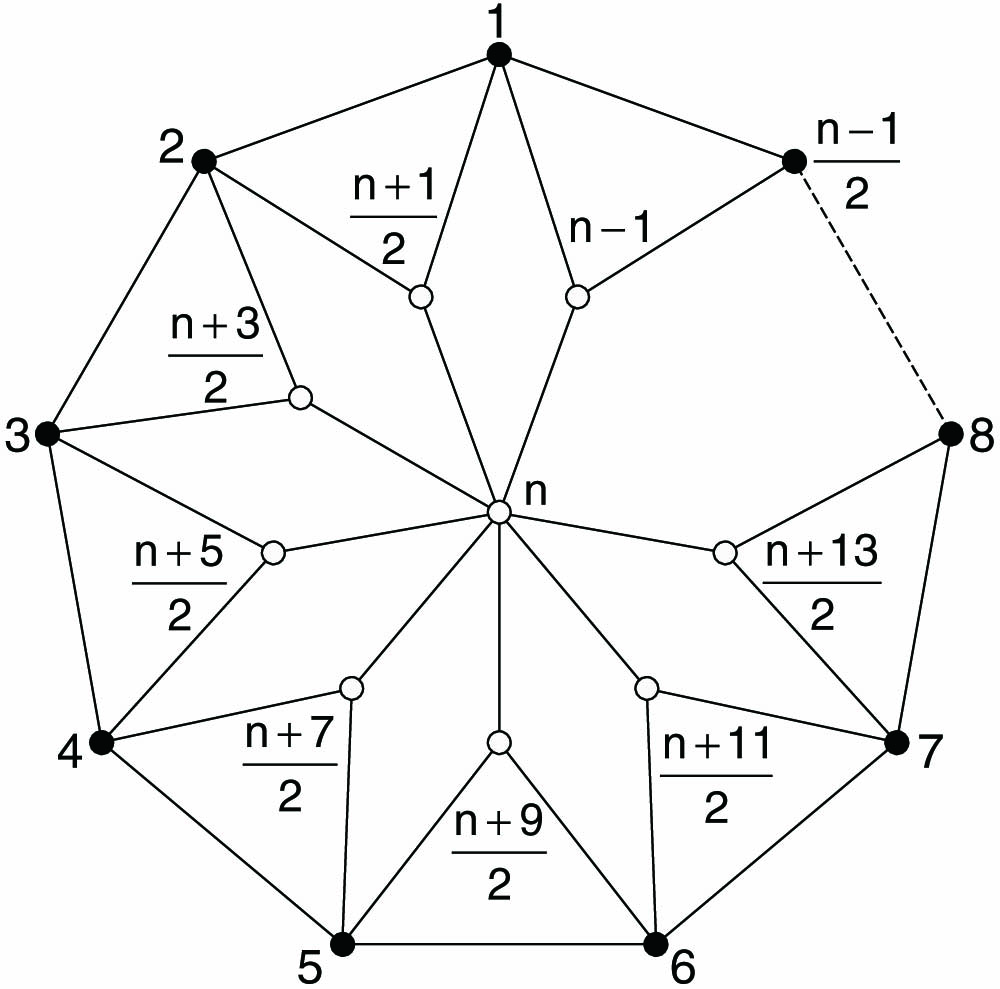
Wen-Rong Qi1、2、†, Jie Zhou3、†, Ling-Jun Kong4、5、†, Zhen-Peng Xu6, Hui-Xian Meng3, Rui Liu1, Zhou-Xiang Wang1, Chenghou Tu1, Yongnan Li1、8、*, Adán Cabello7, Jing-Ling Chen3、9、*, and Hui-Tian Wang4、10、*
Author Affiliations
  • 1Key Laboratory of Weak-Light Nonlinear Photonics and School of Physics, Nankai University, Tianjin 300071, China
  • 2School of Physics, Henan Normal University, Xinxiang 453007, China
  • 3Theoretical Physics Division, Chern Institute of Mathematics, Nankai University, Tianjin 300071, China
  • 4National Laboratory of Solid State Microstructures, Nanjing University, Nanjing 210093, China
  • 5Collaborative Innovation Center of Advanced Microstructures, Nanjing University, Nanjing 210093, China
  • 6Naturwissenschaftlich-Technische Fakultät, Universität Siegen, 57068 Siegen, Germany
  • 7Departamento de Física Aplicada II, Universidad de Sevilla, E-41012 Sevilla, Spain
  • 8e-mail: liyongnan@nankai.edu.cn
  • 9e-mail: chenjl@nankai.edu.cn
  • 10e-mail: htwang@nju.edu.cn
  • show less
    DOI: 10.1364/PRJ.452704 Cite this Article Set citation alerts
    Wen-Rong Qi, Jie Zhou, Ling-Jun Kong, Zhen-Peng Xu, Hui-Xian Meng, Rui Liu, Zhou-Xiang Wang, Chenghou Tu, Yongnan Li, Adán Cabello, Jing-Ling Chen, Hui-Tian Wang. Stronger Hardy-like proof of quantum contextuality[J]. Photonics Research, 2022, 10(7): 1582 Copy Citation Text show less
    Exclusivity graph of the n measurements (with n=7, 11,15, 19, …) used for the Hardy-like proof of contextuality. Each vertex represents a measurement. Vertices connected by an edge are jointly measurable. Each of the outer vertices belongs to two triangles. In total, there are (n−1)/2 triangles.
    Fig. 1. Exclusivity graph of the n measurements (with n=7,11,15,19,) used for the Hardy-like proof of contextuality. Each vertex represents a measurement. Vertices connected by an edge are jointly measurable. Each of the outer vertices belongs to two triangles. In total, there are (n1)/2 triangles.
    Exclusivity relations between the projection measurements in the Hardy-like proof for n=7, including the added measurements (8, 9, 10) used in the experiment. The black vertices are twice of the white vertices in weight.
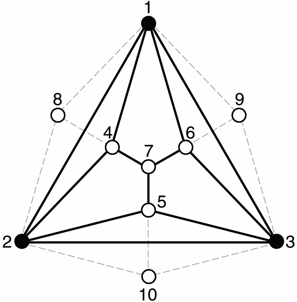
    Fig. 2. Exclusivity relations between the projection measurements in the Hardy-like proof for n=7, including the added measurements (8, 9, 10) used in the experiment. The black vertices are twice of the white vertices in weight.
    Experimental setup. In the state preparation part, a 405 nm cw laser pumps a type-II ppKTP crystal (not shown) to create photon pairs. One photon serves as a trigger. The other photon is projected into the horizontal polarization state with a polarizing beam splitter (PBS); the spatial light modulator (SLM) combines a Rochi grating (RG) through two 4f systems to generate the ququart subset of OAM. In the projection measurement part, two sets of q-plates (QPs, with different topological charges of q1=1/2 and q2=1) are sandwiched by two quarter-wave plates (QWPs), followed by a half-wave plate (HWP) and a PBS used to convert OAM mode into a fundamental mode that is coupled into a single mode fiber (SMF); the photons are detected by a single photon avalanche photodiode (SPAD).
    Fig. 3. Experimental setup. In the state preparation part, a 405 nm cw laser pumps a type-II ppKTP crystal (not shown) to create photon pairs. One photon serves as a trigger. The other photon is projected into the horizontal polarization state with a polarizing beam splitter (PBS); the spatial light modulator (SLM) combines a Rochi grating (RG) through two 4f systems to generate the ququart subset of OAM. In the projection measurement part, two sets of q-plates (QPs, with different topological charges of q1=1/2 and q2=1) are sandwiched by two quarter-wave plates (QWPs), followed by a half-wave plate (HWP) and a PBS used to convert OAM mode into a fundamental mode that is coupled into a single mode fiber (SMF); the photons are detected by a single photon avalanche photodiode (SPAD).
    Quantum violation of Eq. (3) for n=7. NCHV (=3) represents the classical bound of the NCHV theory. The maximum violation is QT1≈3.372 by using the optimal measurement settings, and the non-maximum violation is QT2=3.250 by using the measurements adopted in the Hardy-like proof.
    Fig. 4. Quantum violation of Eq. (3) for n=7. NCHV (=3) represents the classical bound of the NCHV theory. The maximum violation is QT13.372 by using the optimal measurement settings, and the non-maximum violation is QT2=3.250 by using the measurements adopted in the Hardy-like proof.
    Success probabilities PSUC (blue curve) and PCBCB (red curve) versus n.
    Fig. 5. Success probabilities PSUC (blue curve) and PCBCB (red curve) versus n.
    Curve of the ratio rn versus n. The red curve represents the relationship of rn with n in our paper, while the blue curve represents the relationship of rn′ with n for the extended KCBS noncontextuality inequality.
    Fig. 6. Curve of the ratio rn versus n. The red curve represents the relationship of rn with n in our paper, while the blue curve represents the relationship of rn with n for the extended KCBS noncontextuality inequality.
    Different regions for αn, where pi are boundary points, p1=(0,0),p2=(0,2/(n−1)), and p3=(2,1).
    Fig. 7. Different regions for αn, where pi are boundary points, p1=(0,0),p2=(0,2/(n1)), and p3=(2,1).
    Experimental results for δ(_,0|oj,ok) (red circles) and δ(0,_|oj,ok) (black squares) in (a) and for δ(_,1|oj,ok) (red circles) and δ(1,_|oi,oj) (black square) in (b). The numbers of 1 to 24 (even numbers are not marked in figures) represent the settings of (o1,o2), (o1,o3), (o1,o4), (o1,o6), (o2,o1), (o2,o3), (o2,o4), (o2,o5), (o3,o1), (o3,o2), (o3,o5), (o3,o6), (o4,o1), (o4,o2), (o4,o5), (o4,o7), (o5,o2), (o5,o3), (o5,o7), (o6,o1), (o6,o3), (o6,o7), (o7,o4), (o7,o5), and (o7,o6). Error bars are calculated from the counting statistics.
    Fig. 8. Experimental results for δ(_,0|oj,ok) (red circles) and δ(0,_|oj,ok) (black squares) in (a) and for δ(_,1|oj,ok) (red circles) and δ(1,_|oi,oj) (black square) in (b). The numbers of 1 to 24 (even numbers are not marked in figures) represent the settings of (o1,o2), (o1,o3), (o1,o4), (o1,o6), (o2,o1), (o2,o3), (o2,o4), (o2,o5), (o3,o1), (o3,o2), (o3,o5), (o3,o6), (o4,o1), (o4,o2), (o4,o5), (o4,o7), (o5,o2), (o5,o3), (o5,o7), (o6,o1), (o6,o3), (o6,o7), (o7,o4), (o7,o5), and (o7,o6). Error bars are calculated from the counting statistics.
    |ϕ|ν1|ν2|ν3|ν4|ν5|ν6|ν7|ν8|ν9|ν10
    121000120120012
    120100012120120
    120011200121200
    1200012121212121212
    Table 1. State |ϕ and the Measurement Vectors |νj (j=1,2,  ...,  7), Where |ν8,|ν9,|ν10 Are Annex Measurement Vectors
    ProjectorsExperimentIdeal
    o10.248±0.0050.25
    o20.246±0.0040.25
    o40.495±0.0080.50
    o10.247±0.0060.25
    o30.247±0.0050.25
    o60.495±0.0070.50
    o20.247±0.0050.25
    o30.246±0.0060.25
    o50.495±0.0050.50
    o70.248±0.0060.25
    Table 2. Experimental Results of Hardy-Like Proof for n=7a
    Wen-Rong Qi, Jie Zhou, Ling-Jun Kong, Zhen-Peng Xu, Hui-Xian Meng, Rui Liu, Zhou-Xiang Wang, Chenghou Tu, Yongnan Li, Adán Cabello, Jing-Ling Chen, Hui-Tian Wang. Stronger Hardy-like proof of quantum contextuality[J]. Photonics Research, 2022, 10(7): 1582
    Download Citation