Stronger Hardy-like proof of quantum contextuality

Wen-Rong Qi; Jie Zhou; Ling-Jun Kong; Zhen-Peng Xu; Hui-Xian Meng; Rui Liu; Zhou-Xiang Wang; Chenghou Tu; Yongnan Li; Adán Cabello; Jing-Ling Chen; Hui-Tian Wang

doi:10.1364/PRJ.452704

Abstract

A Hardy-like proof of quantum contextuality is a compelling way to see the conflict between quantum theory and noncontextual hidden variables (NCHVs), as the latter predict that a particular probability must be zero, while quantum theory predicts a nonzero value. For the existing Hardy-like proofs, the success probability tends to 1/2 when the number of measurement settings

n

goes to infinity. It means the conflict between the existing Hardy-like proof and NCHV theory is weak, which is not conducive to experimental observation. Here we advance the study of a stronger Hardy-like proof of quantum contextuality, whose success probability is always higher than the previous ones generated from a certain

n

-cycle graph. Furthermore, the success probability tends to 1 when

n

goes to infinity. We perform the experimental test of the Hardy-like proof in the simplest case of

n = 7

by using a four-dimensional quantum system encoded in the polarization and orbital angular momentum of single photons. The experimental result agrees with the theoretical prediction within experimental errors. In addition, by starting from our Hardy-like proof, one can establish the stronger noncontextuality inequality, for which the quantum-classical ratio is higher with the same

n

, which provides a new method to construct some optimal noncontextuality inequalities. Our results offer a way for optimizing and enriching exclusivity graphs, helping to explore more abundant quantum properties.

1. INTRODUCTION

Ideal measurements yield the same outcome when repeated, even when other compatible measurements have been performed in between. Some predictions of quantum theory for ideal measurements cannot be explained under the assumption that ideal measurements reveal preexisting outcomes that are independent of the context (i.e., the set of compatible measurements that have been jointly measured), this is known as quantum contextuality or Kochen–Specker (KS) contextuality [1]. Quantum contextuality is an intrinsic signature of nonclassicality as its classical simulation requires memory [2] and thermodynamical cost [3]. Moreover, it has been proven that quantum contextuality is necessary for fault-tolerant quantum computation via magic state distillation and measurement-based quantum computation [4]. Quantum contextuality also plays a fundamental role in some quantum key distribution protocols [5] and is crucial for understanding the underlying physics behind the limitation of quantum correlations [6]. So far, quantum contextuality has been experimentally observed in trapped ions [7], photons [8], ensembles of molecular nuclear spins in the solid state [9], and superconducting systems [10].

KS contextuality is the first theory about contextuality. The KS-type proof [1,11,12] serves as a no-go theorem, indicating that it is impossible for the noncontextual hidden variable (NCHV) models to describe quantum mechanics. For instance, for Peres-33 rays [11], it is impossible to define any consistent assignment of 0s and 1s to the states in the set. In other words, the standard KS sets cannot be colored in a consistent way in classical theory. Beyond all doubt, the KS-type proof is an elegant argument for contextuality, which is similar to the Greenberger–Horne–Zeilinger (GHZ) proof for the Bell nonlocality. Throughout research history, many well-known scientists have done excellent work on KS contextuality. The first proof scheme of KS includes 117 ray quantities in three-dimensional space, and that with less rays is found step by step [11 –14]. Those that we are familiar with are Peres-33 rays [11], CEG-18 rays [12], and so on. There are some that also have other famous research, for example, the Peres–Mermin square—a considerable simplification of the original KS argument by Mermin and Peres using nine observables that are organized in a $3 \times 3$ square [15,16]. Later, noncontextuality inequality has been proposed as an experiment-friendly approach to reveal quantum contextuality and has been tested by many experiments [7,12,14,17,18]. We will talk about noncontextuality inequality in detail in the next paragraph. In general, a KS-type proof must be transferred to a noncontextuality inequality to be experimentally validated, and experimental tests of contextuality based on standard KS-type proofs were seldom performed in the literature, which may be due to this reason: noncontextuality inequalities are straightforward for the Klyachko–Can–Binicioğlu–Shumovsky (KCBS) cases [19], but in the KS case, the meaning is less clear because value assignments are logically inconsistent, and it is not clear how to compare them with quantum prediction.

The graph-theoretic approach to quantum correlations bridges a fundamental connection between graph theory and quantum contextuality [20,21]. The central idea is that, for an arbitrary exclusivity graph, [Note: Any graph $G (V, E)$ is made up by vertices and edges, where $V$ is a set of vertices and $E$ is the set of edges. The exclusivity graph described that the measurement events $e_{i}$ are represented as the vertices $i$ of the graph, and there is an edge between vertex $i$ and vertex $j$ if events $e_{i}$ and $e_{j}$ are mutually exclusive events, and the corresponding measurement vectors $| v_{i} ⟩$ and $| v_{j} ⟩$ are mutually orthogonal.] one can always associate it with a noncontextuality inequality, for which the classical bound has a definite meaning as the independence number of the graph, and the maximum quantum violation of the inequality is the Lovász number describing the Shannon capacity of the graph. The noncontextuality inequality is a correlation inequality that any theory should satisfy under the assumption of outcome noncontextuality for ideal measurements. The typical examples are the KCBS inequality [12] and its extensions [22] and some state-independent-contextuality (SIC) inequalities [14,23]. The noncontextuality inequalities have these advantages: (i) theoretically, quantum contextuality can be revealed in a direct way by the violations of noncontextuality inequalities; (ii) compared with the KS-type proofs, the violations of noncontextuality inequalities are more feasible to observe quantum contextuality in the experiments.

Sign up for Photonics Research TOC. Get the latest issue of Photonics Research delivered right to you！Sign up now

A natural result yielded from the graph-theoretic approach is the so-called “Hardy-like proof” [24], which for quantum contextuality is analogous to Hardy’s proof for Bell nonlocality [25] and is also a particularly compelling way to reveal contextuality. A Hardy-like proof of contextuality may be seen as a particular violation of the noncontextuality inequality, which is more experimentally friendly than noncontextuality inequalities sometimes. The first Hardy-like proof of contextuality was proposed in Ref. [24] by studying the $n$ -cycle graphs. In such a proof, the NCHV theory predicts that the success probability $P_{SUC}$ of a particular event must be zero, while quantum theory predicts a nonzero value. For the simple Hardy-like proof of the five-cycle graph, $P_{SUC} = 1 / 9$ has been experimentally observed [26]. Remarkably, for the $n$ -cycle graphs, $P_{SUC}$ tends to 1/2 when the number of measurement settings $n$ goes to infinity [24]. The conflict between the simple Hardy-like proof and NCHV theory has not reached the limit. A natural question is whether there is a Hardy-like proof for a certain $n$ -vertex graph, in which $P_{SUC}$ tends to 1 when $n \to \infty$ , thus providing the stronger quantum contextuality.

In this work, a Hardy-like proof was presented for the graphs with $n = 4 m + 3$ $(m = 1, 2, \dots)$ vertices, in which the success probability tends to 1 when the number of measurement settings goes to infinity. For a fixed $n$ , the new Hardy-like proof is stronger than the previous one for the $n$ -cycle graph. To illustrate our idea, we experimentally test the Hardy-like proof with $P_{SUC} = 1 / 4$ in the simplest case of $n = 7$ , by using a four-dimensional quantum system encoded in the polarization and orbital angular momentum (OAM) of single photons. For some symmetric graphs, by starting from the Hardy-like proofs, one can establish some stronger noncontextuality inequalities, for which the quantum-classical ratio is higher or optimal, and this provides a novel way to construct some useful noncontextuality inequalities.

2. STRONGER HARDY-LIKE PROOF

Considering $n = 4 m + 3$ $(m = 1, 2, \dots)$ ideal measurements represented in quantum theory by the rank-one projectors and with possible outcomes 0 and 1, some of these measurements are jointly measurable, while some of the corresponding events are mutually exclusive. The $n$ -vertex exclusivity graph is shown in Fig. 1. Supposing that there is a state $| ϕ ⟩$ ( $ρ = | ϕ ⟩ ⟨ ϕ |$ ), its probabilities for the triangles in Fig. 1 satisfy the following Hardy-like constraints: $\sum_{j = 1,2, \frac{n + 1}{2}} P (τ_{j} ρ | ρ) = 1, \sum_{j = 2,3, \frac{n + 3}{2}} P (τ_{j} ρ | ρ) = 1, ⋮ \sum_{j = 1, \frac{n - 1}{2}, n - 1} P (τ_{j} ρ | ρ) = 1,$ (1)i.e., the sum of the probabilities of each triangle is 1. $(τ_{j} ρ | ρ)$ is the event corresponding to outcome 1 obtained for the measurement $τ_{j}$ in the state $| ϕ ⟩$ , no matter which other compatible measurements are performed. Under these assumptions, any NCHV theory predicts that the outcome of the measurement corresponding to the vertex in the center of Fig. 1 must be zero. That is to say, the NCHV theory predicts $P (τ_{n} ρ | ρ) = 0$ . This is due to the fact that, in the NCHV theory, Eq. (1) implies that at least one of the events that are mutually exclusive with $(τ_{n} ρ | ρ)$ has happened for any given hidden variable. Thus, the event $(τ_{n} ρ | ρ)$ can never happen whatever the hidden variable is, i.e., $P (τ_{n} ρ | ρ) = 0$ . In addition, for the odd number ( $\frac{n - 1}{2} = 2 m + 1$ ) outer vertices in the polygon, not all of those values can be zero; hence, at least one of the inner values has to be 1, and vertex $n$ must be a value of 0. See Appendix A for a detailed proof for the NCHV value of the Hardy-like paradox.

Exclusivity graph of the n measurements (with n=7, 11,15, 19, …) used for the Hardy-like proof of contextuality. Each vertex represents a measurement. Vertices connected by an edge are jointly measurable. Each of the outer vertices belongs to two triangles. In total, there are (n−1)/2 triangles.

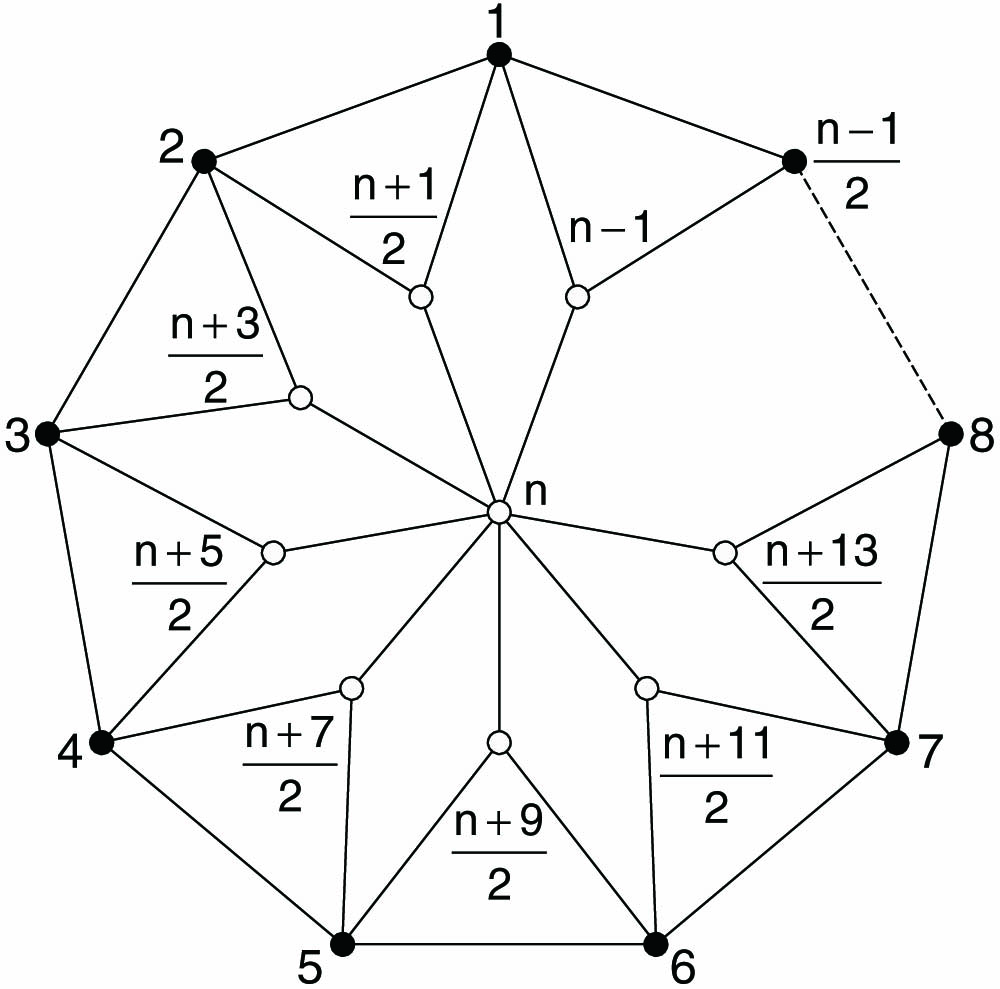
Figure 1.Exclusivity graph of the $n$ measurements (with $n = 7, 11,15, 19, \dots$ ) used for the Hardy-like proof of contextuality. Each vertex represents a measurement. Vertices connected by an edge are jointly measurable. Each of the outer vertices belongs to two triangles. In total, there are $(n - 1) / 2$ triangles.

In contrast, quantum theory predicts that for a four-dimensional quantum state, when $n$ measurements satisfy Eq. (1), the success probability could be $P_{SUC} \equiv P (τ_{n} ρ | ρ) = \cos^{2} (\frac{2 π}{n - 1}) .$ (2)Clearly, the probability tends to 1 when $n \to \infty$ and is 1/4 for the simplest case of $n = 7$ . Moreover, the probability is very close to 1 even for a relatively small $n$ [e.g., for $n = 83$ , $P (τ_{83} ρ | ρ) \approx 0.994$ ]. The state and the measurement vectors for $P (τ_{n} ρ | ρ)$ are listed in Table 3 (see Appendix B), and the detailed comparison of $P (τ_{n} ρ | ρ)$ with the success probability obtained in the $n$ -cycle Hardy-like proof [24] is shown in Table 4 (see Appendix C).

Table 1 lists the state $| ϕ ⟩$ and the corresponding projectors $τ_{j} = | ν_{j} ⟩ ⟨ ν_{j} |$ , and we have $P (τ_{n} ρ | ρ) = 1 / 4$ for $n = 7$ . The exclusivity relations between the projection measurements are given by the graph in Fig. 2. In addition, three annex points (denoted by $| ν_{8} ⟩, | ν_{9} ⟩, | ν_{10} ⟩$ ) are added due to the need of experimental test for the compatibility conditions.Table 1.

State $| ϕ ⟩$ and the Measurement Vectors $| ν_{j} ⟩$ ( $j = 1, 2, ..., 7$ ), Where $| ν_{8} ⟩, | ν_{9} ⟩, | ν_{10} ⟩$ Are Annex Measurement Vectors

$\| ϕ ⟩$	$\| ν_{1} ⟩$	$\| ν_{2} ⟩$	$\| ν_{3} ⟩$	$\| ν_{4} ⟩$	$\| ν_{5} ⟩$	$\| ν_{6} ⟩$	$\| ν_{7} ⟩$	$\| ν_{8} ⟩$	$\| ν_{9} ⟩$	$\| ν_{10} ⟩$
$\frac{1}{2}$	1	0	0	0	$\frac{1}{\sqrt{2}}$	0	$\frac{1}{2}$	0	0	$\frac{1}{\sqrt{2}}$
$\frac{1}{2}$	0	1	0	0	0	$\frac{1}{\sqrt{2}}$	$\frac{1}{2}$	0	$\frac{1}{\sqrt{2}}$	0
$\frac{1}{2}$	0	0	1	$\frac{1}{\sqrt{2}}$	0	0	$\frac{1}{2}$	$\frac{1}{\sqrt{2}}$	0	0
$\frac{1}{2}$	0	0	0	$\frac{1}{\sqrt{2}}$	$\frac{1}{\sqrt{2}}$	$\frac{1}{\sqrt{2}}$	$- \frac{1}{2}$	$- \frac{1}{\sqrt{2}}$	$- \frac{1}{\sqrt{2}}$	$- \frac{1}{\sqrt{2}}$

Figure 2.Exclusivity relations between the projection measurements in the Hardy-like proof for $n = 7$ , including the added measurements (8, 9, 10) used in the experiment. The black vertices are twice of the white vertices in weight.

3. STRONGER NONCONTEXTUALITY INEQUALITY

Every Hardy-like proof of quantum contextuality can be considered as a violation of a noncontextuality inequality [24]. Hence, a Hardy-like proof can be used as the starting point for identifying new noncontextuality inequalities. An interesting issue is identifying situations in which few measurement settings can produce a high degree of contextuality. The issue is of great importance for applications in which the degree of contextuality has one-to-one correspondence with the quantum-versus-classical advantage [27]. To characterize the degree of quantum contextuality, it is defined as the ratio between the maximum quantum violation and the noncontextual bound [27]. When performing an operation by the Hardy-like proof presented above, we select the weights of the vertices in the symmetric graph (Fig. 1) for achieving the optimal degree of quantum contextuality. Thus, we obtain the following noncontextuality inequality as $I_{n} = 2 \sum_{j = 1}^{\frac{n - 1}{2}} P (τ_{j} ρ | ρ) + \sum_{j = \frac{n + 1}{2}}^{n} P (τ_{j} ρ | ρ) \overset{NCHV}{\leq} \frac{n - 1}{2} .$ (3)This inequality is violated by the quantum state in the four-dimensional quantum system. Notice that, in Fig. 1, black vertices have a weight of 2 while white vertices have a weight of 1 in Eq. (3). For $n = 7$ , the noncontextual bound of $I_{n}$ is 3, while the maximum quantum violation is $(1 + \sqrt{33}) / 2 \approx 3.372$ . This maximum violation can be achieved by the state $| ψ ⟩ = {(α, α, α, β)}^{T}$ , and the measurements correspond to the projectors onto the seven vectors of $| ν_{1} ⟩ = {(1,0,0,0)}^{T}$ , $| ν_{2} ⟩ = {(0,1,0,0)}^{T}$ , $| ν_{3} ⟩ = {(0,0,1,0)}^{T}$ , $| ν_{4} ⟩ = {(0,0, γ, ζ)}^{T}$ , $| ν_{5} ⟩ = {(γ,0,0, ζ)}^{T}$ , $| ν_{6} ⟩ = {(0, γ,0, ζ)}^{T}$ $| ν_{7} ⟩ = {(μ, μ, μ, ε)}^{T}$ , where $α = \sqrt{(11 + 5 \sqrt{33}) / 132}$ , $β = \sqrt{(33 - 5 \sqrt{33}) / 44}$ , $γ = \sqrt{(9 - \sqrt{33}) / 8}$ , $ζ = \sqrt{(\sqrt{33} - 1) / 8}$ , $μ = \sqrt{2 / 3} γ$ , $ε = - \sqrt{(\sqrt{33} - 5) / 4}$ (see Appendix D for the cases of higher $n$ ).

Equation (3) has remarkable properties, as follows. (i) For any $n$ , Eq. (3) leads to a higher degree of contextuality than the one obtained by the extended KCBS noncontextuality inequality (see Appendix E). The extended KCBS inequality is the default target inequality in the contextuality experiment [26] and is also the inequality that naturally follows from the Hardy-like proof in Ref. [24]. (ii) For the simplest case ( $n = 7$ ), numerical computation shows that the inequality (3) leads to a higher degree of contextuality than other noncontextuality inequalities in form $\sum_{j = 1}^{7} w_{j} ⟨ P_{j} ⟩ \leq C$ , where $w_{j}$ is the weight of the rank-one projector $P_{j}$ for the $j$ th vertex, and $C$ is the classical bound. For $n = 7$ , the maximum degree of contextuality for the extended KCBS inequality is 1.106 [22], while for inequality $I_{7} \leq 3$ , it is 1.124. For some of the discussions, see Appendix F. This property reveals that searching for situations, in which a few measurement settings lead to a high degree of contextuality, may be beneficial for investigating symmetric graphs and attributing different weights to each of the classes of vertices.

4. EXPERIMENTAL RESULTS

The new Hardy-like proof and the corresponding inequality can reveal the contextuality in a new system because they provide better contextuality witnesses than the extended KCBS inequality under the same number of measurement settings. We will test the Hardy-like proof (for the simplest case of $n = 7$ ) in a hybrid four-dimensional quantum system defined by the polarization and OAM of single photons. Testing contextuality is especially difficult as sequential measurements are not easy to implement. To overcome this difficulty, a simple method (which needs two measurements only) has been presented, in which the first measurement can be simulated by a demolition measurement followed by a preparation that depends on the outcome [28]. Of course, the necessary no-signaling conditions [29] also need to be satisfied. Based on this method, in order to test the Hardy-like proof in Eqs. (1) and (2) for $n = 7$ , we should add mutually orthogonal vertices to form complete sets. Figure 2 shows that ${1,2,4,8}, {1,3,6,9}$ , and ${2,3,5,10}$ have formed three complete sets.

The experimental setup (Fig. 3) consists of two parts: the state preparation and the projection measurement. In the state preparation, photon pairs are produced via a type-II spontaneous parametric downconversion in a 10-mm-long periodically poled potassium titanyl phosphate (ppKTP) crystal pumped by a 405 nm cw ${TEM}_{00}$ diode laser, and one photon serves as a trigger. The produced photons can carry the discrete OAM of $l ℏ$ [30] ( $l$ is an arbitrary integer, and $ℏ$ is the reduced Planck constant). Therefore, high-dimensional information can be encoded in the OAM of single photons [31]. As the original work on OAM [32], we consider an OAM carried by Laguerre–Gaussian (LG) mode of azimuthal $l$ order and radial order $p = 0$ in our experiment. Equally weighted superpositions of LG modes with different OAMs ( $l_{1} ℏ$ and $l_{2} ℏ$ ), and the relative phase $ξ$ can be written as ${LG}_{l_{1}, l_{2}} (r, φ) = \frac{1}{\sqrt{2}} [{LG}_{l_{1}} (r, φ) + e^{i ξ} {LG}_{l_{2}} (r, φ)] .$ (4)

Figure 3.Experimental setup. In the state preparation part, a 405 nm cw laser pumps a type-II ppKTP crystal (not shown) to create photon pairs. One photon serves as a trigger. The other photon is projected into the horizontal polarization state with a polarizing beam splitter (PBS); the spatial light modulator (SLM) combines a Rochi grating (RG) through two 4f systems to generate the ququart subset of OAM. In the projection measurement part, two sets of $q$ -plates (QPs, with different topological charges of $q_{1} = 1 / 2$ and $q_{2} = 1$ ) are sandwiched by two quarter-wave plates (QWPs), followed by a half-wave plate (HWP) and a PBS used to convert OAM mode into a fundamental mode that is coupled into a single mode fiber (SMF); the photons are detected by a single photon avalanche photodiode (SPAD).

We generate the ququart states based on the interferometric superposition of horizontally (H) and vertically (V) polarized photons carrying OAMs, which is similar to that in Ref. [33]. The collimated photons at 810 nm are split into two paths by a beam splitter (BS). Two computer-generated holographic gratings (HG1 and HG2) displayed on a spatial light modulator (SLM) ( $1920 \times 1080 pixels$ ) diffract the H-polarized light into different diffraction orders. Then a Rochi grating (RG) is used to recombine the $- 1$ st diffraction order of HG1 and the $+ 1$ st diffraction order of HG2 into the single one, as shown in Fig. 3. The weight and phase of two different OAMs can be controlled by adjusting the HGs. Thus, we use the two-dimensional orthogonal polarizations and four-dimensional OAMs ( $l = \pm 1$ and $\pm 3$ ) to build four-dimensional subspace ${| H, + 1 ⟩, | V, - 1 ⟩, | H, + 3 ⟩, | V, - 3 ⟩}$ . Finally, the prepared state can be expressed as follows: $| ϕ ⟩ = \frac{1}{2} (| H, + 1 ⟩ + | V, - 1 ⟩ + | H, + 3 ⟩ + | V, - 3 ⟩) .$ (5)

In the projection measurement, we perform the projection measurements by two $q$ -plates (QPs) with topological charges of $q_{1} = 1 / 2$ and $q_{2} = 1$ , respectively. The function of the QP can be described as $| L, l ⟩ \overset{QP}{\to} | R, l + 2 q ⟩$ , $| R, l ⟩ \overset{QP}{\to} | L, l - 2 q ⟩$ [34], where $L$ and $R$ denote left- and right-handed circular polarizations, respectively. Two cascaded QPs sandwiched between two quarter-wave plates (QWPs) are used to convert $| ν_{j} ⟩$ into a ${TEM}_{00}$ mode, which is easily coupled to a single photon avalanche photodiode (SPAD) through the single mode fiber (SMF).

In order to measure the probability for $n = 7$ in Eq. (2), we need to introduce two additional vertices ( $a$ , $b$ ) to form a complete set ${5,7, a, b}$ , where $| ν_{a} ⟩ = \frac{1}{\sqrt{2}} {(0,1, - 1, 0)}^{T}$ and $| ν_{b} ⟩ = \frac{1}{2} {(- 1,1,1, - 1)}^{T}$ . Here we describe the observables by $o_{j} = | ν_{j} ⟩ ⟨ ν_{j} |$ . For the sake of simplicity, $P (τ_{j} ρ | ρ)$ is replaced by $P (1 | o_{j})$ . We first perform the verification of no-signaling between two measurements. We use the equations given in Ref. [22] to characterize the influence, $δ (_,0 | o_{j}, o_{k}) = | P (0 | o_{k}) - P (0,0 | o_{j}, o_{k}) - P (1,0 | o_{j}, o_{k}) |, δ (_,1 | o_{j}, o_{k}) = | P (1 | o_{k}) - P (0,1 | o_{j}, o_{k}) - P (1,1 | o_{j}, o_{k}) |,$ which represent the statistical effects of the first measurement on the second measurement, indicating that the result of projecting the state onto $o_{k}$ is 0 and 1, respectively. In the same way, the statistical effects of the second measurement on the first should be $δ (0,_| o_{j}, o_{k}) = | P (0 | o_{j}) - P (0,0 | o_{j}, o_{k}) - P (0,1 | o_{j}, o_{k}) |, δ (1,_| o_{j}, o_{k}) = | P (1 | o_{j}) - P (1,0 | o_{j}, o_{k}) - P (1,1 | o_{j}, o_{k}) | .$ To obtain $P (0,1 | o_{j}, o_{k})$ , we need to prepare the orthogonal state $| ν_{j}^{⊥} ⟩$ based on the Lüder rule [35]. Our experiment meets the no-signaling condition within the experimental accuracy, $δ (_,0 | o_{j}, o_{k}) \approx δ (0,_| o_{j}, o_{k}) = 0$ and $δ (_,1 | o_{j}, o_{k}) \approx δ (1,_| o_{j}, o_{k}) = 0$ (see Appendix G). The projection probability and the joint measurement probability should be measured in their corresponding complete sets.

Figure 4.Quantum violation of Eq. (3) for $n = 7$ . NCHV ( $= 3$ ) represents the classical bound of the NCHV theory. The maximum violation is $QT 1 \approx 3.372$ by using the optimal measurement settings, and the non-maximum violation is $QT 2 = 3.250$ by using the measurements adopted in the Hardy-like proof.

5. CONCLUSION

Stronger quantum contextuality is particularly significant as it reveals a sharper contradiction between the NCHV theory and the quantum theory. In this work, we have advanced the study of a stronger Hardy-like proof of quantum contextuality. We have theoretically presented a new Hardy-like proof, which is stronger than the previous one given in Ref. [24]. For the simplest case ( $n = 7$ ), the success probability equals 1/4, and it tends to 1 when $n \to \infty$ . We have also performed the experimental test for the new Hardy-like proof by the four-dimensional quantum system encoded in the polarization and OAM of single photons. The experimental result gives $P_{SUC} = 0.248 \pm 0.006$ , which agrees with the theoretical prediction within the experimental errors. Importantly, the stronger Hardy-like proof can yield stronger noncontextuality inequality and has an advantage over the extended KCBS noncontextuality inequality for the $n$ -cycle graphs. Our results not only advance the study of the Hardy-like proof for quantum correlations but also open a new approach to observe quantum contextuality in new systems. That also paves a way for further research on fundamental quantum resources.

APPENDIX A: PROOF FOR THE NCHV VALUE FOR THE HARDY-LIKE PARADOX

P_{i}

P_{i} = \sum_{y \in Λ} p (y) ℘_{i} (y),

P_{1} + P_{2} + P_{\frac{n + 1}{2}} = 1, P_{2} + P_{3} + P_{\frac{n + 3}{2}} = 1, ⋮ P_{1} + P_{\frac{n - 1}{2}} + P_{n - 1} = 1 .

APPENDIX B: MEASUREMENTS OF THE STATE FOR THE HARDY-LIKE PROOF OF QUANTUM CONTEXTUALITY WITH n MEASUREMENTS

n

| ν_{j} ⟩

APPENDIX C: COMPARISON BETWEEN THE SUCCESS PROBABILITIES PSUC AND PCBCB

n

P_{SUC}

Figure 5.Success probabilities $P_{SUC}$ (blue curve) and $P_{CBCB}$ (red curve) versus $n$ .

P_{SUC}

APPENDIX D: STATE AND MEASUREMENTS FOR THE MAXIMUM QUANTUM VALUE OF In

n = 4 m + 3 (m = 1, 2, \dots)

Quantum State $| ψ ⟩$ and Measurements $τ_{j}$ $(j = 1, 2, \dots, n)$ , for the Maximum Quantum Value of $I_{n}$ ^a

$\| ν_{1} ⟩$	1	0	$λ \sin θ$	$λ \cos θ$
$\| ν_{2} ⟩$	$\cos (t)$	$\sin (t)$	$λ \sin θ$	$λ \cos θ$
$\| ν_{3} ⟩$	$\cos (2 t)$	$\sin (2 t)$	$λ \sin θ$	$λ \cos θ$
$⋮$	$⋮$	$⋮$	$⋮$	$⋮$
$\| ν_{\frac{n - 1}{2}} ⟩$	$\cos (\frac{n - 3}{2} t)$	$\sin (\frac{n - 3}{2} t)$	$λ \sin θ$	$λ \cos θ$
$\| ν_{\frac{n + 1}{2}} ⟩$	$κ λ \sin θ \cos (\frac{t}{2})$	$κ λ \sin θ \sin (\frac{t}{2})$	1	0
$\| ν_{\frac{n + 3}{2}} ⟩$	$κ λ \sin θ \cos (\frac{3 t}{2})$	$κ λ \sin θ \sin (\frac{3 t}{2})$	1	0
$\| ν_{\frac{n + 5}{2}} ⟩$	$κ λ \sin θ \cos (\frac{5 t}{2})$	$κ λ \sin θ \sin (\frac{5 t}{2})$	1	0
$⋮$	$⋮$	$⋮$	$⋮$	$⋮$
$\| ν_{n - 1} ⟩$	$κ λ \sin θ \cos (\frac{n - 2}{2} t)$	$κ λ \sin θ \sin (\frac{n - 2}{2} t)$	1	0
$\| ν_{n} ⟩$	0	0	0	1
$\| ψ ⟩$	0	0	$\cos x$	$\sin x$

Here $τ_{j}$ are the projectors onto the vectors $| ν_{j} ⟩$ (non-normalized) and $ρ = | ψ ⟩ ⟨ ψ |$ , $t = (n - 3) π / (n - 1)$ , $k = - 1 / \cos (t / 2)$ , and $λ = \sqrt{\cos [2 π / (n - 1)]}$ .

Table 6.

Numerical Value of Quantum Bound^a

$n$	7	11	15	19	23	27	31
$θ$	$\frac{1}{2} \arccos [(\sqrt{33} - 7) / 2]$	0.269	0.198	0.158	0.131	0.112	0.098
$x$	$\frac{1}{2} \arccos [- \sqrt{(23 - 4 \sqrt{33}) / 11}]$	1.106	1.219	1.285	1.329	1.362	1.386
$Q_{n}$	$\frac{1}{2} (\sqrt{33} + 1)$	5.730	7.849	9.903	11.932	13.950	15.962
$n$	35	39	43	63	83	103
$θ$	0.087	0.079	0.071	−0.049	−0.037	0.030
$x$	1.406	1.421	1.434	1.666	1.644	1.512
$Q_{n}$	17.970	19.975	21.980	31.990	41.994	51.996

For the optimal values of the parameters $θ$ and $x$ , one can obtain the maximum quantum violation $Q_{n}$ in Eq. (D1).

Q_{n}

APPENDIX E: COMPARISON OF DEGREE OF QUANTUM CONTEXTUALITY BETWEEN OUR INEQUALITY AND THE EXTENDED KCBS INEQUALITY

r_{n} = \frac{Q_{n}}{α_{n}},

I_{n}^{'} = \sum_{j = 1}^{n} P (0,1 | j, j + 1) \overset{NCHV}{⩽} α_{n}^{'} \overset{QT}{⩽} Q_{n}^{'},

r_{n}^{'} = \frac{Q_{n}^{'}}{α_{n}^{'}} = \frac{2 n \cos (π / n)}{(n - 1) [1 + \cos (π / n)]} .

r_{n}

Numerical Values of the Ratios $r_{n}$ and $r_{n}^{'}$ with $n$ for the Inequalities in Eqs. (D1) and (E2)

$n$	5	7	11	15	19	23	27	31	35	39	43	63	83	103
$r_{n}$	–	1.124	1.146	1.121	1.100	1.085	1.073	1.064	1.057	1.051	1.047	1.032	1.024	1.020
$r_{n}^{'}$	1.118	1.106	1.077	1.060	1.048	1.041	1.035	1.031	1.027	1.025	1.022	1.016	1.011	1.010

Figure 6.Curve of the ratio $r_{n}$ versus $n$ . The red curve represents the relationship of $r_{n}$ with $n$ in our paper, while the blue curve represents the relationship of $r_{n}^{'}$ with $n$ for the extended KCBS noncontextuality inequality.

n

APPENDIX F: OPTIMAL NONCONTEXTUALITY INEQUALITY WITH WEIGHTS OF c=2 AND d=1

n

c

| ψ ⟩

Figure 7.Different regions for $α_{n}$ , where $p_{i}$ are boundary points, $p_{1} = (0,0), p_{2} = (0,2 / (n - 1))$ , and $p_{3} = (2,1)$ .

n = 7

System.Xml.XmlElementSystem.Xml.XmlElementSystem.Xml.XmlElement

r_{7} (c, d, x, θ) = \frac{Q_{7} (c, d, x, θ)}{α_{7} (c, d)} = \frac{c \sin^{2} (θ + x) + \frac{3 d \cos^{2} (x)}{2 - \cos (2 θ)} + \sin^{2} (x)}{d + c} \leq \frac{c \sin^{2} (θ + x) + \frac{3 d \cos^{2} (x)}{2 - \cos (2 θ)} + \sin^{2} (x)}{3 d} = \frac{c}{3 d} \sin^{2} (θ + x) + \frac{3 d}{3 d} \frac{\cos^{2} (x)}{2 - \cos (2 θ)} + \frac{1}{3 d} \sin^{2} (x) = \frac{c}{3 d} \sin^{2} (θ + x) + \frac{\cos^{2} (x)}{2 - \cos (2 θ)} + \frac{1}{3 d} \sin^{2} (x) .

d

r_{7}

n = 7

n = 7

APPENDIX G: EXPERIMENTAL DETAILS

{LG}_{l_{1}, l_{2}} (r, φ) = \frac{1}{\sqrt{2}} [{LG}_{l_{1}} (r, φ) + e^{i ξ} {LG}_{l_{2}} (r, φ)],

q_{1} = 1 / 2

Efficiencies of the Two Cascaded QPs Sandwiched between Two QWPs

Input State	Output State	Efficiency
$\| H, + 1 ⟩$	$\| H,0 ⟩$	66.9%
$\| V, - 1 ⟩$	$\| H,0 ⟩$	66.8%
$\| H, + 3 ⟩$	$\| H,0 ⟩$	66.5%
$\| V, - 3 ⟩$	$\| H,0 ⟩$	66.7%

δ (_,0 | o_{j}, o_{k}) = | P (0 | o_{k}) - P (0,0 | o_{j}, o_{k}) - P (1,0 | o_{j}, o_{k}) |, δ (_,1 | o_{j}, o_{k}) = | P (1 | o_{k}) - P (0,1 | o_{j}, o_{k}) - P (1,1 | o_{j}, o_{k}) |,

δ (0,_| o_{j}, o_{k}) = δ (1,_| o_{j}, o_{k}) = 0

Figure 8.Experimental results for $δ (_,0 | o_{j}, o_{k})$ (red circles) and $δ (0,_| o_{j}, o_{k})$ (black squares) in (a) and for $δ (_,1 | o_{j}, o_{k})$ (red circles) and $δ (1,_| o_{i}, o_{j})$ (black square) in (b). The numbers of 1 to 24 (even numbers are not marked in figures) represent the settings of $(o_{1}, o_{2})$ , $(o_{1}, o_{3})$ , $(o_{1}, o_{4})$ , $(o_{1}, o_{6})$ , $(o_{2}, o_{1})$ , $(o_{2}, o_{3})$ , $(o_{2}, o_{4})$ , $(o_{2}, o_{5})$ , $(o_{3}, o_{1})$ , $(o_{3}, o_{2})$ , $(o_{3}, o_{5})$ , $(o_{3}, o_{6})$ , $(o_{4}, o_{1})$ , $(o_{4}, o_{2})$ , $(o_{4}, o_{5})$ , $(o_{4}, o_{7})$ , $(o_{5}, o_{2})$ , $(o_{5}, o_{3})$ , $(o_{5}, o_{7})$ , $(o_{6}, o_{1})$ , $(o_{6}, o_{3})$ , $(o_{6}, o_{7})$ , $(o_{7}, o_{4})$ , $(o_{7}, o_{5})$ , and $(o_{7}, o_{6})$ . Error bars are calculated from the counting statistics.

References

[1] S. Kochen, E. P. Specker. The problem of hidden variables in quantum mechanics. J. Math. Mech., 17, 59-87(1967).

[2] A. Cabello, M. Gu, O. Gühne, Z. P. Xu. Optimal classical simulation of state-independent quantum contextuality. Phys. Rev. Lett., 120, 130401(2018).

[3] A. Cabello, M. Gu, O. Gühne, J.-Å. Larsson, K. Wiesner. Thermodynamical cost of some interpretations of quantum theory. Phys. Rev. A, 94, 052127(2016).

[4] M. Howard, J. Wallman, V. Veitch, J. Emerson. Contextuality supplies the ‘magic’ for quantum computation. Nature, 510, 351-355(2014).

[5] A. Cabello, V. D’Ambrosio, E. Nagali, F. Sciarrino. Hybrid ququart-encoded quantum cryptography protected by Kochen-Specker contextuality. Phys. Rev. A, 84, 030302(2011).

[6] B. Yan. Quantum correlations are tightly bound by the exclusivity principle. Phys. Rev. Lett., 110, 260406(2013).

[7] G. Kirchmair, F. Zähringer, R. Gerritsma, M. Kleinmann, O. Gühne, A. Cabello, R. Blatt, C. F. Roos. State-independent experimental test of quantum contextuality. Nature, 460, 494-497(2009).

[8] R. Lapkiewicz, P. Li, C. Schaeff, N. Langford, S. Ramelow, M. Wieśniak, A. Zeilinger. Experimental non-classicality of an indivisible quantum system. Nature, 474, 490-493(2011).

[9] O. Moussa, C. A. Ryan, D. G. Cory, R. Laflamme. Testing contextuality on quantum ensembles with one clean qubit. Phys. Rev. Lett., 104, 160501(2010).

[10] M. Jerger, Y. Reshitnyk, M. Oppliger, A. Potočnik, M. Mondal, A. Wallraff, K. Goodenough, S. Wehner, K. Juliusson, N. K. Langford, A. Fedorov. Contextuality without nonlocality in a superconducting quantum system. Nat. Commun., 7, 12930(2016).

[11] A. Peres. Two simple proofs of the Kochen-Specker theorem. J. Phys. A, 24, L175(1991).

[12] A. Cabello, J. Estebaranz, G. García-Alcaine. Bell-Kochen-Specker theorem: a proof with 18 vectors. Phys. Lett. A, 212, 183-187(1996).

[13] M. Kernaghan, A. Peres. Bell-Kochen-Specker theorem for 20 vectors. J. Phys. A, 27, L829(1994).

[14] S. Yu, C. H. Oh. State-independent proof of Kochen-Specker theorem with 13 rays. Phys. Rev. Lett., 108, 030402(2012).

[15] A. Peres. Incompatible results of quantum measurements. Phys. Lett. A, 151, 107-108(1990).

[16] N. D. Mermin. Simple unified form for the major no-hidden-variables theorems. Phys. Rev. Lett., 65, 3373-3376(1990).

[17] A. Cabello. Experimentally testable state-independent quantum contextuality. Phys. Rev. Lett., 101, 210401(2008).

[18] E. Amselem, M. Rådmark, M. Bourennane, A. Cabello. State-independent quantum contextuality with single photons. Phys. Rev. Lett., 103, 160405(2009).

[19] A. A. Klyachko, M. A. Can, S. Binicioğlu, A. S. Shumovsky. Simple test for hidden variables in spin-1 systems. Phys. Rev. Lett., 101, 020403(2008).

[20] A. Cabello, S. Severini, A. Winter. (Non-)Contextuality of physical theories as an axiom(2010).

[21] A. Cabello, S. Severini, A. Winter. Graph-theoretic approach to quantum correlations. Phys. Rev. Lett., 112, 040401(2014).

[22] G. Cañas, E. Acuña, J. Cariñe, J. F. Barra, E. S. Gómez, G. B. Xavier, G. Lima, A. Cabello. Experimental demonstration of the connection between quantum contextuality and graph theory. Phys. Rev. A, 94, 012337(2016).

[23] I. Bengtsson, K. Blanchfield, A. Cabello. A Kochen–Specker inequality from a SIC. Phys. Lett. A, 376, 374-376(2012).

[24] A. Cabello, P. Badziąg, M. Terra Cunha, M. Bourennane. Simple Hardy-like proof of quantum contextuality. Phys. Rev. Lett., 111, 180404(2013).

[25] L. Hardy. Nonlocality for two particles without inequalities for almost all entangled states. Phys. Rev. Lett., 71, 1665-1668(1993).

[26] B. Marques, J. Ahrens, M. Nawareg, A. Cabello, M. Bourennane. Experimental observation of Hardy-like quantum contextuality. Phys. Rev. Lett., 113, 250403(2014).

[27] B. Amaral, M. Terra Cunha, A. Cabello. Quantum theory allows for absolute maximal contextuality. Phys. Rev. A, 92, 062125(2015).

[28] A. Cabello. Simple method for experimentally testing any form of quantum contextuality. Phys. Rev. A, 93, 032102(2016).

[29] Y. Xiao, Z. P. Xu, Q. Li, J. S. Xu, K. Sun, J. M. Cui, Z. Q. Zhou, H. Y. Su, A. Cabello, J. L. Chen, C. F. Li, G. C. Guo. Experimental observation of quantum state-independent contextuality under no-signaling conditions. Opt. Express, 26, 32-50(2018).

[30] G. Molina-Terriza, J. P. Torres, L. Torner. Twisted photons. Nat. Phys., 3, 305-310(2007).

[31] L. J. Kong, R. Liu, W. R. Qi, Z. X. Wang, S. Y. Huang, Q. Wang, C. Tu, Y. Li, H. T. Wang. Manipulation of eight-dimensional Bell-like states. Sci. Adv., 5, eaat9206(2019).

[32] L. Allen, M. W. Beijersbergen, R. J. C. Spreeuw, J. P. Woerdman. Orbital angular momentum of light and the transformation of Laguerre-Gaussian laser modes. Phys. Rev. A, 45, 8185-8189(1992).

[33] X. L. Wang, J. P. Ding, W. J. Ni, C. S. Guo, H. T. Wang. Generation of arbitrary vector beams with a spatial light modulator and a common path interferometric arrangement. Opt. Lett., 32, 3549-3551(2007).

[34] L. Marrucci, E. Karimi, S. Slussarenko, B. Piccirillo, E. Santamato, E. Nagali, F. Sciarrino. Spin-to-orbital conversion of the angular momentum of light and its classical and quantum applications. J. Opt., 13, 064001(2011).

[35] G. Lüders. Über die zustandsänderung durch den meßprozeß. Ann. Phys., 8, 322-328(1951).

Input State	Output State	Efficiency
$\| H, + 1 ⟩$	$\| H,0 ⟩$	66.9%
$\| V, - 1 ⟩$	$\| H,0 ⟩$	66.8%
$\| H, + 3 ⟩$	$\| H,0 ⟩$	66.5%
$\| V, - 3 ⟩$	$\| H,0 ⟩$	66.7%