Conventional optical imaging techniques work under the condition that spherical wavelets emitting from a target to the entrance pupil cannot be severely distorted.¹ Otherwise, they cannot converge after passing through the lens system and form the image. However, in applications ranging from in situ biomedical inspection in life sciences² to free space optical communication in cloudy and hazy environments,³ this condition is not satisfied when scattering media exist between the target and the optical system, distorting the propagation direction of each wavelet in a random manner. When the distortion is weak, one can use adaptive optical techniques to measure it and compensate.⁴ However, when the distortion is strong, no image can be formed as the photons are scattered many times randomly inside the medium. The photon-scattering process is explicitly deterministic (described by the so-called scattering matrix) when the scattering medium is static, meaning that it is reversible.⁵ Taking advantage of this property, many efforts have been made to exploit imaging through scattering media using either optical or computational techniques. In the optical domain, Goodman et al. have demonstrated that one can measure the scattered wavefront distortion by using holography.⁶ Holography has been extended to produce a phase-conjugated beam of the scattered one⁷ so that the distortion can be removed when the beam propagates back through the scattering medium once again, and to separate the ballistic photons by taking the advantage of coherence gating.⁸ Furthermore, it has been demonstrated that holography has the potential to image a three-dimensional object behind a thin diffuser.⁹ Nevertheless, holography only records the complex wavefront of the beam that leaves the scattering medium, without any information about the scattering process occurring inside. Alternatively, wavefront shaping has been proposed to actively control the propagation of the beam through the scattering medium.^10–12 This can be phenomenologically interpreted as the control of the photons so that a certain amount of them can make their way through the scattering medium in the eigenchannels. In this way, wavefront shaping can be used to measure the transmission matrix (TM) of scattering media,¹³ allowing the transmission of images through opaque media.¹⁴ However, the state-of-the-art spatial light modulators (SLMs) can neither shape the complex-valued wavefront precisely nor measure the TM at the wavelength scale of a scattering medium of large volume due to the pixel size and count, which imposes a limitation to the powerful wavefront-shaping technique. Memory effect,¹⁵ on the other hand, promises noninvasive¹⁶ and single-shot imaging through a scattering layer,^17,18 and has been widely explored recently.¹⁹ However, the memory effect range of the light field that passes through the scattering slab drops very quickly to the wavelength scale as the slab becomes thicker,²⁰ imposing a strict limitation on the field of view of the scattering imaging system.^17,21

Here, we exploit the technique of deep learning and develop a special hybrid neural network (HNN) architecture for imaging through optically thick scattering media. It is well known that machine learning techniques including deep learning have been widely employed to solve the problems in recognition and classification.^22,23 It was not until recently that researchers started to use them in the field of computational imaging.^24–32 Horisaki et al.²⁴ proposed to use the support vector regression architecture to reconstruct the scattering images with a set of human face data for training. Lyu et al.²⁵ were the first to use deep learning for imaging through scattering media. Li et al.³⁰ proposed to use a convolutional neural network (CNN) to achieve coherent imaging through thin ground glass, and Li et al.³¹ proposed to use a residual neural network that is highly scalable to both scattering medium perturbations and measurement requirements. However, the works reported in Refs. 29 and 30 dealt with thin scattering layers like ground glass, through which the relationship between the acquired speckle and the target is easy to model owing to the memory effect. This is not the case when the scattering media become optically thick. In a previous study,²⁵ we have demonstrated how to solve this problem with deep neural network (DNN) architecture. But there were three big issues when we applied it in imaging through a thick scattering wall. First, in a DNN, every neuron in one hidden layer is usually connected to every other neuron in the immediate downstream layer, resulting in a parametric space that is time-consuming to optimize. Second, even though the training can converge eventually, overfitting is very likely to occur.^25,33 Third, the trained network is hard to generalize. In this paper, we demonstrate that the above drawbacks can be overcome using an HNN model. In the conceptual demonstration, we develop an HNN that can retrieve the coherent images of various targets behind a 3-mm-thick white polystyrene slab from the corresponding speckle pattern acquired with a digital camera. Furthermore, our experimental results suggest that the speckle pattern contains redundant information, as the target image can be reconstructed from as little as 0.1% information content possessed by the acquired speckle pattern. This suggests great potential for the compression and storage of the information-carrying speckle patterns and their transmission through wired or wireless communication channels.

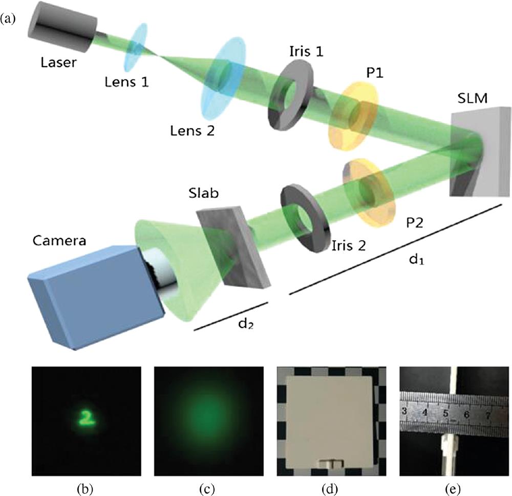
The optical setup used in our experiments is schematically illustrated in Fig. 1(a). The laser we used was a linearly polarized optically pumped semiconductor laser (Verdi G2 SLM, Coherent Inc.) irradiating at 532 nm. A collimated and expanded laser beam was shone on an amplitude-only liquid crystal SLM after passing through the linear polarizer P1 and Iris 1, which were used to control the polarization state and width of the beam. The amplitude-only SLM was a Holoeye Pluto-Vis with a maximum pixel count of 1920×1080 and a pixel size of 8.0μm×8.0μm. The target images were displayed on the SLM to modulate the incident beam. The targets we used were images of handwritten digits from the MNIST database³⁴ with a size of 28×28pixels. We first resized these images 18 times to 504×504 and zero-padded them to 1920×1080 before displaying them on the SLM. As a result, the physical size of the handwritten digit was about 2mm×2mm (calculated by counting the number of pixels used to represent the digits). The image-carrying beam reflected from the SLM was then shone onto a 3-mm-thick white polystyrene slab (EDU-VS1/M, Thorlabs Inc.), after a distance d1=290mm of propagation in free space. At the other side of the slab, a camera (Andor Zyla 4.2 PLUS sCMOS with a 4.2-megapixel sensor) was placed at a distance d2=35mm to collect the speckle pattern generated by light scattering inside the slab. To obtain amplitude modulation, we placed a linear polarizer P2 whose polarization direction was perpendicular with respect to P1 in the reflected beam. An iris (Iris 2) was also used, to select the first-order reflection. In the experiments, we activated only the central 512×512pixels of the camera for speckle data acquisition.

To visually display the scattering power of the 3-mm-thick polystyrene slab, we first project an image directly on the front surface of the slab, and see how it looks at the back surface. The results are shown in Figs. 1(b) and 1(c), respectively. As can be seen, the image is very clear at the front surface but becomes highly diffusive at the other side of the slab, in contrast to the case of passing through thin ground glass.^16,17 This is because the light has been scattered many times on the way through the slab. Indeed, the measured optical depth of the scattering slab is about 13.40 (see Appendix A), so the light is in the diffusive regime.²

Nevertheless, the speckle pattern I captured by the camera is related to the target O through the TM.³⁵ Our purpose is then to retrieve the target image O from the speckle pattern I. Note that, for weak scattering layers such as a ground glass, their relation is reduced to the convolution U(R)=∫O(r)h(r;R)d2r, where R measures the position on the surface of camera sensor and r measures the position on the surface of the SLM, within the isoplanatic angle. The captured speckle pattern I(R)=U(R)U(R)*. The memory effect¹⁶ allows us to reconstruct the target image by phase retrieval because the autocorrelation of I is approximately equal to the autocorrelation of |O|2. However, when the scattering medium is sufficiently thick, as in our study, the memory effect is destroyed and the isoplanatic angle tends to zero.³⁶ This means that the spherical wavelets emitted from any two points of a target, although separated by a very small distance, will effectively experience two distinct scattering processes, resulting in two elemental speckle patterns that are totally uncorrelated. One can imagine that the final speckle pattern corresponding to the whole target is produced by the superposition of many of these uncorrelated elemental patterns. As a consequence, one will not expect that an image of the target can be reconstructed using the memory-effect-based techniques. In the case of imaging through static scattering media, one may choose to use TM-based techniques,^13,14 because the TM is deterministic. However, it is unfeasible in our case here, because the TM should be measured in the wavelength scale and across a large area, whereas current SLM technologies are not ready for that yet.

The deep-learning-based method that we propose here to image through optically thick media is a data-driven solution. This means that we need a large set of input–output measurements to train the neural network model so as to learn how the speckle patterns are related to the targets.

Even though the universal approximation theorem^37,38 states that a two-layer network can uniformly approximate any continuous function to arbitrary accuracy, such a two-layer network will require a huge amount of neurons, making it difficult to train. Therefore, a neuron network with more layers and fewer neurons in each layer is more favorable. Note that a typical CNN architecture is translation equivariance.²² But the system we are encountering now becomes spatially variant due to the presence of the thick scattering medium. As a result, attempting to build a spatially invariant neural network to mimic a spatially variant imaging system will take a lot of effort. On the contrary, a fully connected network such as the DNN can be spatially variant. But the training is usually time-consuming and the resulting network architecture is hard to generalize as aforementioned.^25,33 It typically takes many hours or even days to train depending on the size of the training set and the geometry of the network. For example, the fully connected DNN model that we developed for imaging through scattering²⁵ took us 18 h to train with a Tesla K20c GPU. Thus, an HNN composed of a few layers of DNN and a few layers of CNN is more desirable.

The HNN architecture we report here has five two-dimensional (2-D) convolutional layers, two reshaping layers, one pooling layer, three densely connected layers, and five dropout layers, as schematically shown in Fig. 2. The three densely connected layers were sandwiched between the five convolutional layers, two upstream and three downstream. For demonstration, we arbitrarily took a block of 64×64pixels out of each 512×512-pixels speckle pattern acquired by the camera as the input to the network. The two upstream layers were used to extract 32 feature maps of the input speckle, resulting in a 32×32×32-pixel feature cube. Then it was reshaped to a 1×32,768 vector and served as the input to the three sequential densely connected layers, which has 1024, 784, and 784 neurons, respectively. Then another reshaping layer r2 was used to shape the 1×784 vector back to a 28×28-pixel image for the sake that we could use the raw handwritten digits from the MNIST database directly to calculate the loss function. Three 2-D convolutional layers with the kernel of 3×3, 2×2, and 1×1pixels, respectively, were used to calculate the feature maps in three different abstraction levels. The output of the network was a 28×28-pixel image. In the proposed HNN, the activation function was the rectified linear units,³⁹ which allowed fast and effective training of the network compared with the sigmoid.³⁸ We used the mean square error (MSE) as the loss function, and Adam⁴⁰ as the strategy to update the weights in the training process. To reduce overfitting, dropout layers⁴¹ were used throughout the HNN architecture.

To train the HNN, we used images of 3990 handwritten digits downloaded from the MNIST handwritten digit database³⁴ as the training sets. In the experiment, we sequentially displayed them on the amplitude-only SLM shown in Fig. 1 and captured the corresponding speckle patterns. As aforementioned, we used only the central 512×512pixels of the sCMOS camera for data acquisition. More specifically, the training set was created by pairing up the 3990 28×28-pixel handwritten digits with the corresponding 64×64 speckle patterns, which were randomly taken out of the 512×512 speckle patterns acquired by the camera. The set of 3990 pairs’ input–output data was fed into the HNN model to optimize the connection weights and biases of all the neurons. The program was implemented on the Keras framework with Python 3.5, and sped up by a GPU (NVIDIA Quadro P6000). The training was converged after only 1 epoch of about 194 s. The time it took to reconstruct an image from its speckle was 0.78 s in our experiment.

To test the performance, we experimentally obtained 10 speckle patterns corresponding to 10 other digits from the MNIST database but not in the training set and sent them to the trained neural network. These 10 test speckle patterns are shown in Fig. 3(a). The images reconstructed by the proposed HNN are shown in Fig. 3(b). In comparison with the ground-truth images shown in Fig. 3(c), all the visible features, and particularly the edges of the targets, have been retrieved successfully. Unlike the images reconstructed using the phase conjugation,⁷ wavefront shaping,^10,11 or transmission matrix,¹³ the background of the images retrieved using the HNN is very clean. We also plot the images reconstructed using the memory-effect-based method in Fig. 3(d) for comparison. One can see that nothing but noise is reconstructed in this case. This result is expected, and consistent with the theoretical prediction,¹⁵ as the range of memory effect is about 0.01 deg measured by using the standard technique,^20,35 whereas the angular extent of the digits displayed on the SLM is about 0.4 deg.

Usually, a neural network produces a better result if the feature of a test image is closer to that of the training images.²⁷ Surprisingly, in the case of imaging through thick scattering media, we found that the HNN trained by the digital images alone can retrieve the images of handwritten English letters, which were manually written by one of the authors. The experimentally reconstructed results are shown as the five letter columns [right-hand side of Fig. 3(b)].

Now let us compare the proposed HNN with the CNN and DNN architectures in terms of imaging performance. To do that, we first need to make a CNN and a DNN. For the sake of fairness in comparison, all the networks should have the same number of layers, even though it is not possible to make them the same width. Thus, we changed the three densely connected layers in the proposed HNN to convolutional layers and made it a CNN and changed all the convolutional layers to the densely connected layers to establish a DNN. The 10 reconstructed test images are shown in Fig. 4. One can see from the results that the DNN can reconstruct the handwritten digits with an acceptable quality (except the digit “5”), but it failed in the case of English letters. This means that the trained DNN has limited generalization. The CNN performed even worse, as only the digit “6” can be reconstructed.

It is instructive to understand where the information of the target is stored in the speckle patterns and how well it can be compressed. To quantify our analysis, we first define the information content (IC) according to Shannon’s information theory:⁴²IC=nplog2(Ns),(1)where np is the total number of image elements (pixels), and Ns is the signal’s distinguishable intensity level, which is represented by gmax−gmin, where gmax and gmin are the maximum gray level and minimum gray level of the captured images. For most of the speckle patterns captured by the camera np=512×512; gmax=216−1=65,535; and gmin=16,729 instead of 0, because they were not regularized with respect to the background.

It is well known that holograms contain the whole wavefront of the objects.¹ Even a small fraction can reconstruct the object wavefront, although noise arises. In the case of coherent imaging through a thick scattering medium, the speckle acquired by the camera is formed by the interference of light taking many possible paths inside the medium. The motivation here is to study if the speckle formed by the diffusive light holds the same property. In fact, since we only use part of raw scattering images, it is suggested that our neural network can reconstruct the object from partial information. We arbitrarily select three small blocks (marked by a1, a2, and a3) of 64×64pixels out of each captured raw speckle patterns of 512×512 to train the HNN network, as shown in Fig. 5. The results are shown in Fig. 6. It is clearly seen that both the digits and the English letters are retrieved successfully, although there are some distortions in the results of English letters.

Surprisingly, we could even randomly pick 4096 pixels, not necessarily in a continuous block, out of each raw speckle pattern, and arbitrarily arrange them to form a new 64×64 speckle-like pattern. Then, we paired it up with the associated handwritten digit, although they are not directly physically related to each other. Following the same process (picking the pixels at the same positions and rearranging them in the same way), we obtained 3990 pair data of this type and used them to train the HNN. Then, we generated some test speckle patterns in the same way and used them to test the HNN. The results, as shown in Fig. 7, suggest that the information about the target does spread across the whole speckle pattern, similarly to the hologram. And it does not matter which part of the recorded speckle pattern is used.

A significant concern is to determine how small the fraction of the speckle can be to faithfully reconstruct the target image. To explore this possibility, we took out blocks of six different sizes (8×8, 16×16, 32×32, 64×64, 128×128, and 256×256) from each speckle pattern and paired them up with the corresponding targets to train the network. Of course, the network width should be changed accordingly, since the size of the input speckle that the network will process is different. When the networks were well trained, we used them to process the test speckle patterns of the corresponding size; the reconstructed images are shown in Fig. 8. The results suggest that as the size of speckle reduces, the quality of the reconstructed image degrades. Specifically, the reconstructed image is still recognizable if the input speckle is 32×32pixels. But the reconstructed image is severely distorted when we use only 256 or fewer pixels of the recorded speckle.

The results suggest that the speckle pattern produced in this way is indeed highly redundant. The information of the target is actually encoded everywhere across the speckle pattern.

Now we go further to see if it is possible to reconstruct the image by using less bit depth from the 64×64-pixel subspeckle pattern. The sCMOS camera we used has a bit depth of 16 bits, quantifying the pixel value of the speckle pattern to the range of 0 to 65,535. We examined the effect in two ways. First, we only used a subrange of the pixel value of the test speckle patterns to reconstruct the target images. For example, we used the pixels with the values in the range of 25,000 to 30,000, setting the value of the pixel to 0 if it is <25,000 and to 65,535 if it is >30,000, and as-is if it is in the range of 25,000 to 30,000. The reconstructed results are shown in Fig. 9(G1). One can see that it is distorted in both the cases of handwritten digits and English letters. Similarly, when we used the pixels in the range of 35,000 to 40,000 and 40,000 to 45,000 as the input, we have the results that are shown in Figs. 9(G2) and 9(G3), respectively. One can see that the reconstructed digits are recognizable, whereas the English letters are distorted, suggesting the limited ability of generalization in this case. The difference in quality between the images reconstructed using the pixels in different ranges is mainly due to the probability density function of the speckle intensity.⁴³ Since the pixel values are mainly in the range of 25,000 to 45,000, we are unable to reconstruct the target images by using the pixels whose values are below 25,000 or above 45,000 alone. Second, we examined an extreme case of binarizing the test speckle patterns by setting all the pixel values <35,000 to 0, and otherwise to 65,535. Experimental results show that the target images can be reconstructed even in this case, as shown in the Fig. 9(G4).

The results presented in Secs. 4.2.1 and 4.2.2 suggest that the speckle patterns generated in this way are highly redundant and therefore compressible in both the spatial and the bit depth domains. To measure the redundancy of the speckle pattern, we can calculate the information content according to Eq. (1). For the raw speckle pattern directly captured by the camera, the information capacity is IC=(512×512)log2(65,535−16,729)≈4.1×106bits. And for the speckle patterns of minimal size and bit depth that contain sufficient information to reconstruct the target image with acceptable quality, the information content is reduced to IC=(64×64)log2(2)=4096bits. Thus the compression ratio is given as C=40964.1×106≈0.1%.(2)This means that only 0.1% of the information contained by the captured speckle pattern is sufficient to reconstruct the target image with the proposed HNN.

From the information theory point of view, this result is reasonable because the information content of the handwritten digits is <4096. But no other method except properly designed neural networks can be used to reconstruct the target image from such a small fraction of the recorded speckle, to the best of our knowledge.

We have proposed a deep learning method for imaging through thick scattering media. Specifically, we experimentally demonstrated the faithful reconstruction of a image of the target hidden behind a 3-mm-thick polystyrene slab with an optical depth of 13.4. The proposed HNN architecture is composed of fully connected layers and convolutional layers so that it has the advantages of both the DNN and the CNN, and thus gives better performance. As a learning-based method, it requires a large set of labeled data for training. But it just needs to be trained once. The collection of the training data set is also required for the techniques of wavefront shaping and TM measurement. But the requirement of the training data in the proposed method is not as strict as in the other two, which should be a set of spatial modes¹⁵ in wavefront shaping, and a set of plane waves with different spatial frequencies³⁶ in the TM method. In addition, it does not need to measure the complex amplitude but only the input–output intensities so that the experimental system can be more simple and concise. Furthermore, it does not need to use any microscopic objective to demagnify the images displayed on the SLM to fit the size of the eigenchannel.^11,15 This means that the trained HNN may not reveal any physical details about the transmission matrix of the scattering slab. Nevertheless, it opens up a new possibility for exploring optical imaging through more general complex systems. Finally, we have also demonstrated that the speckle patterns acquired by the camera are highly redundant. Experimentally, we demonstrated that the use of only 0.1% of the information content of the captured speckle pattern is sufficient to reconstruct the target image, meaning that the information-carrying speckle is highly compressible.

The optical depth ds of scattering sample is defined as⁴⁴where Ib is the intensity of the ballistic light and Ii is the intensity of the incident light. We used the experimental system shown in Fig. 10 to measure the optical depth. Two variable irises with the diameter D=8mm were used to adjust the size of the beam. The distance d between the slab and the power meter was 600 mm. First, we measured the incident power Ii to be 8.599 mW. This was done without the slab. Then, we measured the scattered light power Is=17.32nW by placing the slab in the light path. Finally, we placed a metal plate behind Iris 2, in order to block the ballistic light, and measured the background noise In=4.05nW. Then, the ballistic light Ib=Is−In=13.27nW. In our experiments, the optical depth of the white polystyrene slab is 13.40, according to Eq. (3).