Deep learning-based scattering removal of light field imaging

Weihao Wang; Xing Zhao; Zhixiang Jiang; Ya Wen

doi:10.3788/COL202220.041101

Abstract

Light field imaging has shown significance in research fields for its high-temporal-resolution 3D imaging ability. However, in scenes of light field imaging through scattering, such as biological imaging in vivo and imaging in fog, the quality of 3D reconstruction will be severely reduced due to the scattering of the light field information. In this paper, we propose a deep learning-based method of scattering removal of light field imaging. In this method, a neural network, trained by simulation samples that are generated by light field imaging forward models with and without scattering, is utilized to remove the effect of scattering on light fields captured experimentally. With the deblurred light field and the scattering-free forward model, 3D reconstruction with high resolution and high contrast can be realized. We demonstrate the proposed method by using it to realize high-quality 3D reconstruction through a single scattering layer experimentally.

Keywords

computational imaging deep learning light field imaging scattering imaging

1. Introduction

Light field (LF) imaging technology has shown great significance in recent years for its high-temporal-resolution 3D imaging feature through simultaneously capturing the 2D spatial and 2D angular information of light [four-dimensional (4D) LF information]^[1–5]. Especially, the LF imaging method based on the wave-optics model and LF point spread function (LFPSF) allows 3D deconvolution for the high-quality single-shot volumetric reconstruction^[6,7]. However, in some applications of LF imaging, a scattering medium is present in the scenes, such as biological tissue, fog, and turbid water^[8–16]. In these imaging scenes, signal light could still be captured, and 3D reconstruction could be conducted, but scattered light produced by the scattering medium introduces blur and scattering background artifacts to the 3D reconstruction image, which lead to low resolution and low contrast. For the LF imaging method based on 3D deconvolution, sequence recorded frames are utilized to extract ballistic light and undo the effect of scattering on the LF in real-time localization of neuronal activity^[10,11], but the demand of multiple frames rather than single-shot reduced the flexibility of the method. Signal light and scattered light are separated and reconstructed separately^[14], but this will increase the amount of calculation and the solving difficulty. In a general method, scattering is incorporated into the LF imaging forward model to deal with the case of mismatching between the scattering-free model and the LF with scattering, and then the scattering background artifacts of 3D reconstruction can be removed^[8,9]. However, scattering introduces degradation of the LF image and produces blur patterns of LFPSF. These make the inverse problem of the 3D deconvolution more ill-conditioned and lead to a noise-sensitive result^[17].

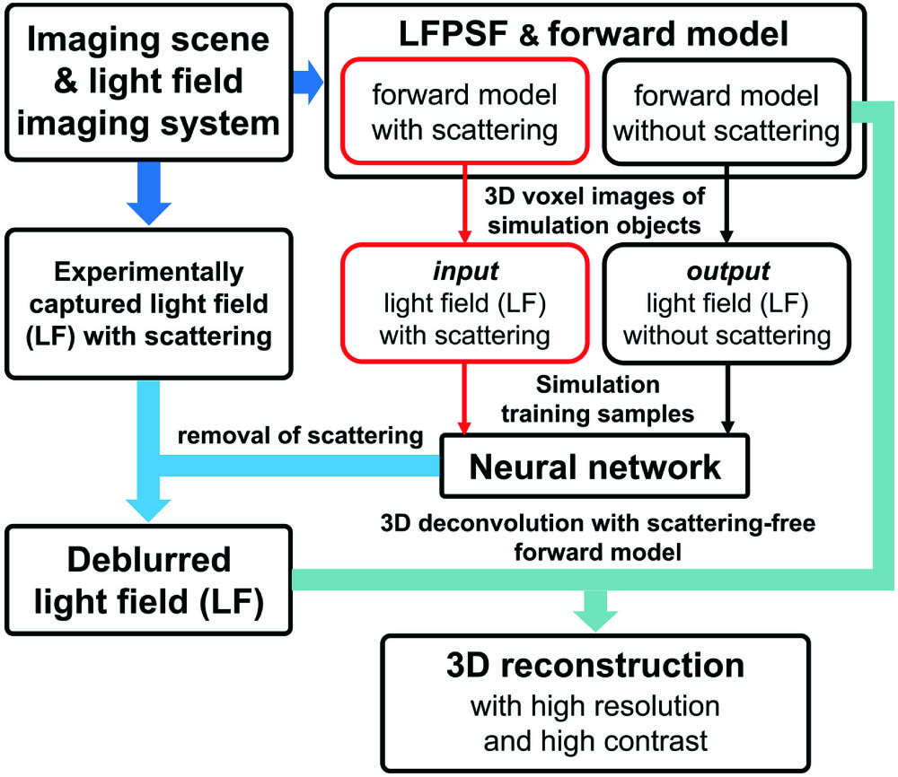
In recent years, deep learning has been widely studied due to its remarkable ability in information processing and has shown great value in the field of computational imaging^[18–24], especially in LF imaging^[25,26] and scattering imaging^[27–30].

In this paper, a deep learning-based method of removal of the scattering effect on LF imaging is proposed to deal with the case of scattering imaging in LF imaging applications mentioned above. We term this method deep learning-based scattering LF imaging (DeepSLFI). In DeepSLFI, we build the LF imaging forward models and generate training samples of LF images with and without scattering by simulation. By the means of simulation, the huge experimental workload for samples capturing can be avoided. Then, a neural network trained with the simulation samples is utilized to remove the effect of scattering on the LF image captured experimentally. Finally, the high-resolution and high-contrast 3D reconstruction can be conducted with the processed LF image. In this paper, a validation experiment is conducted, and the 3D reconstructions of the scene of imaging through a single scattering layer are obtained. Compared to the results of conventional methods, the 3D reconstruction using DeepSLFI has a higher quality in terms of resolution and contrast.

Sign up for Chinese Optics Letters TOC. Get the latest issue of Chinese Optics Letters delivered right to you！Sign up now

2. Method

The overview of DeepSLFI is shown in Fig. 1. The building of the LF imaging forward model is conducted with the theory of LF imaging^[6–9,31]. The LFPSFs and the forward model, shown in Fig. 2, which refer to the projection of the 3D volume in the object space to the 2D image space on the sensor, can be obtained with the determined scene and imaging system. The discretized forward model can be expressed as a matrix equation, $f = H g,$ (1)where $f$ represents the LF image captured by the sensor, $g$ is the object space volume to be reconstructed, and $H$ is the measurement matrix determined by the LFPSFs (reflecting the light propagation). The element $h_{i j}$ in row $j$ of column $i$ in $H$ is $h_{i j} = \iint_{α_{j}, β_{i}} I (x, p) d p d x,$ (2)which refers to the proportion of the light arriving at pixel $j$ propagating from emitters in voxel $i$ , where $I (x, p)$ is the intensity at $x = (x_{1}, x_{2})$ on the sensor, responding to the light emitted from the point emitter located at $p = (p_{1}, p_{2}, p_{3})$ , $α_{j}$ is the area for pixel $j$ , and $β_{i}$ is the volume for voxel $i$ ^[6]. Generally, a micro-lens array (MLA) is utilized to encode the 3D intensity distribution of the volumetric object into LF information and determine the LFPSFs.

Figure 1.Overview of DeepSLFI. The light field imaging forward models can be built after the scattering imaging scene and the light field imaging system are determined. The simulation light field images serving as training samples can be generated with the forward models. Then, a neural network will be trained with the samples and utilized to remove the scattering of the light field image captured experimentally. Finally, the high-resolution and high-contrast 3D reconstruction can be obtained by 3D deconvolution with the deblurred light field image and the scattering-free forward model.

Figure 2.Diagram of light field imaging forward model. Light emitted from voxels of object space g propagates to the sensor. The intensity distribution f on the sensor plane is the light field image. The column of H means light field point spread function (LFPSF), which is the proportion on the sensor of light emitted from the corresponding voxel of object space. With the f captured experimentally, g can be obtained by solving the inverse problem of the equation.

In the absence of scattering, light propagation can be described by theories of wave optics and Fresnel propagation^[6,7,31]. The wavefront at $x = (x_{1}, x_{2}, x_{3})$ of light emitted from the point emitter located at $p = (p_{1}, p_{2}, p_{3})$ is $U (x, p) = \frac{1}{r} \exp (i k r),$ (3)where $k$ is the wave number, and $r = {‖ p - x ‖}_{2}$ . Fresnel propagation can be expressed by the Fourier transform operator $F {•}$ as $U_{output} (x) = F^{- 1} {F {U_{input} (x)} \exp [- \frac{i}{4 π} λ d (ω_{x}^{2} + ω_{y}^{2})]},$ (4)where $U_{output}$ and $U_{input}$ are the wavefront of output plane and input plane (after and before propagation), respectively, $λ$ is the wavelength in the vacuum, $d$ is the propagation distance, and $ω_{x}$ and $ω_{y}$ are spatial frequencies along the $x$ and $y$ directions, respectively. The lens/lenslet and MLA can be modeled as phase masks $ϕ_{lens} (x)$ and $Φ_{MLA} (x)$ , respectively: $ϕ_{lens} (x) = \exp (\frac{- i k}{2 f} {‖ x ‖}_{2}^{2}),$ (5) $Φ_{MLA} (x) = ϕ_{lens} (x) * comb (x / d_{pitch}),$ (6)where $f$ is the focal length of the lens/lenslet of the MLA, $d_{pitch}$ is the pitch of the lenslet of the MLA, $*$ means convolution, and $comb (•)$ is comb function. The intensity on the sensor plane of light is $I_{sensor} (x) = {| U_{sensor} (x) |}^{2}$ .

In the presence of scattering, light propagation can be described by an analysis method based on phase-space theory^[8,9,32]. This allows the scattering to be described with a homogeneous scattering approximation to obtain an analytic forward model, which could not be realized by the theory of Fresnel propagation. The 4D phase-space Wigner function is $W (r, u)$ ^[8], where $r = (x, y)$ is the transverse spatial coordinates, and $u = (u_{x}, u_{y})$ is the spatial frequency coordinates. Then, a 2D intensity image can be described as $I (r) = \iint W (r, u) d^{2} u$ . An incoherence point emitter located at $p = (p_{1}, p_{2}, p_{3})$ could be described by the Wigner function of the plane located on depth $p_{3}$ as $W_{s} (r, u) = δ (r - r_{s})$ , where $r_{s} = (p_{1}, p_{2})$ . The propagation of distance $Δ z$ in Wigner space and the effect of the lens can be modeled as Eqs. (7) and (8), respectively^[32]: $W_{output} (r, u) = \iint W_{input} (r^{'}, u) δ (r - r^{'} - \frac{λ Δ z u}{n_{r}}) d^{2} r^{'},$ (7) $W_{output} (r, u) = \iint W_{input} (r, u^{'}) δ (u - u^{'} + \frac{r}{λ f}) d^{2} u^{'},$ (8)where $W_{output}$ and $W_{input}$ are the Wigner functions of the output plane and input plane, respectively, $r^{'} = (x_{1}^{'}, x_{2}^{'})$ is the spatial coordinates of the input plane, $u^{'} = (u_{x}^{'}, u_{y}^{'})$ is the spatial frequency coordinates of the input plane, and $n_{r}$ is the refractive index. Especially, the intensity at point $r$ on the back focal plane of the lens/lenslet of the MLA can be approximately represented as $I (r) = W (r_{lens}, u_{lens})$ , where $W (r_{lens}, u_{lens})$ is the Wigner function of the lens plane, $r_{lens}$ is the center of the lens/lenslet, and $u_{lens}$ approximately corresponds to $λ u_{lens} / n_{r} = (r - r_{lens}) / f$ . The scattering of the diffusing plane can be described as $W_{output} (r, u) = \iint W_{input} (r, u^{'}) D (u - u^{'}) d^{2} u^{'},$ (9)where $D (u - u^{'})$ is the phase function, which refers to the effect of scattering on directions of the outgoing photons^[33]. A homogeneous scattering approximation is utilized, and the phase function could represent the statical intensity distribution of the outgoing angle information relative to the incident angle information. In Ref. [8], scattering is modeled as an in-place Gaussian spreading of angle information. Here, we propose a modified version of this phase function. The modified version is also based on Gaussian distribution but is more flexible, especially because it can well describe the property of the scattering layer in our experiment later in this paper: $D (u - u^{'}) = \sum_{m} A_{m} \exp [- \frac{{(u - u^{'})}^{2}}{σ_{m}^{2}}], m \in Z^{+},$ (10)where $σ_{m}$ is the scattering coefficient, and $A_{m}$ is the weight factor.

After determining the light propagation in the imaging scene, the intensity proportion on the sensor of the light emitted from point emitter in the object space, $I (x, p)$ , can be calculated by Eqs. (3 )–(10). Then, $H$ and the forward model can be built by Eqs. (1) and (2). With the $H$ and the LF image $f$ captured experimentally, the 3D reconstruction of $g$ can be obtained by solving the inverse problem of the matrix equation through 3D deconvolution. Figure 3 shows the blur and the scattering noise introduced by the scattering layer used in the experiment later in this paper. The signal light could still be captured, but the scattered light would result in serious background artifacts of the 3D reconstruction. Once introducing scattering into the forward model, the blurred LFPSFs would make the inverse problem more ill-conditioned and lead to serious noise sensitivity. These would seriously reduce the quality of 3D reconstruction, especially in a complex scenario.

Figure 3.Light field images captured experimentally of the same object (a) without scattering and (b) with scattering. (a1) and (b1) correspond to the parts of the dashed boxes in (a) and (b), respectively. (c) The intensity curves of pixels on the blue and green lines.

In order to remove the effect of scattering on the LF image, a convolutional neural network (CNN) is used in DeepSLFI. Figure 4 is the overall architecture of the CNN, which is adapted from the residual network (ResNet)^[34] and U-shaped network (U-Net)^[35]. The network consists of eight convolution blocks, each composed of a convolution, a leaky rectified linear unit (LeakyReLU), a batch normalization (BN) layer, and a final tanh activation. The CNN has shown the ability of image deblurring in our preliminary simulation work^[36].

Figure 4.Architecture of the neural network.

Considering the huge workload and the serious difficulty for the experimental capturing of samples of 3D images or LF images in scattering scenes, the training sample pairs will be generated by simulation with the LF imaging forward models. This method also makes DeepSLFI more flexible. The LF imaging forward models have been applied in research^[6–9] and have good performances in describing the practical LF propagation. Therefore, it is believed that the forward models can be utilized to generate samples. Trained with the LF images with scattering (as input) and the scattering-free LF images (as output), the CNN will effectively remove the scattering effect on the input LF image.

The final reconstruction will be realized by 3D deconvolution using the scattering-removed LF image and the scattering-free forward model (which has sharp patterns of LFPSFs). In this paper, CNN is utilized to remove the scattering of the LF image, not to produce 3D image results of the inverse problem end-to-end^[25,26]. The 3D reconstruction will be conducted by an iterative algorithm, such as the Richardson–Lucy algorithm^[6], which is the proven technique, and we are more adept at.

3. Experiment and Results

An experiment is conducted to verify the validity of DeepSLFI. Compared with the 3D reconstruction results obtained from different LF imaging methods, the advantages of DeepSLFI in LF imaging through scattering could be demonstrated.

The experimental system is shown in Fig. 5, which consists of a CCD sensor (BFLY-PGE-50H5M-C, Point Grey, 3.45 µm pixel size and $2 \times 2$ pixels binning employed, the LF image will be a $10 \times 10$ image array with a $730 \times 730$ resolution), an MLA (#64-480, Edmund Optics, 0.5 mm lenslet pitch and 15.3 mm focal length), a lens (focal length 100 mm), a square aperture with the width of 3.27 mm (used to prevent aliasing of subimages of the LF image), and a 0.5 mm thick scattering layer (introduced as a single diffusing plane that can be added or removed as demanded). The imaging object will be a white light source. The wavelength of 632.8 nm is selected to build the forward models. In this experiment, the light mainly propagates in free space, thin optical devices, and thin scattering layer. In addition, the numerical aperture of the system is small. Therefore, the dispersion of the experimental system is very small, and the mismatch between the monochromatic forward models and the white light imaging scene can be ignored. In Ref. [6], the monochromatic forward model also has a good performance in imaging with white light sources.

Figure 5.Diagram of the validation experimental system.

The effect of the scattering layer on the LF image is shown in Fig. 3. Considering that the intensity curves in Fig. 3(c) are smooth in general, and the homogeneous scattering approximation in research of LF imaging through scattering has demonstrated its validity^[8,9], the homogeneous scattering is a very good approximation and will be used in our modeling process. In addition, a homogeneous scattering approximation allows for an analytic forward model for scattering.

By calculating the light intensity distributions on the sensor after the propagation shown in Fig. 6, the LFPSFs and the forward models can be obtained with Eqs. (1 )–(10). A set of parameters of the scattering model, which can well describe the scattering effect of the scattering layer in the experiment, is used. Generally, the effect of aberration can be negligible in the forward model^[6–9,31], especially because the numerical aperture and field of view of the imaging system in this experiment are small. The field of view of the system is a $5.1 mm [height (H)] \times 5.1 mm [width (W)] \times 25 mm [depth (D)]$ cube, where the front plane of the depth of field is 145 mm away from the lens, as shown in Fig. 5. The resolution of the voxel image is $211 (H) \times 211 (W) \times 25 (D)$ , and the sampling rates are uniform at different depths.

Figure 6.Light propagation in the experimental system.

The simulation training samples are generated based on the scene: single-layer planar objects located on 25 depths (1 voxel thickness) with intensity maps of the Modified National Institute of Standards and Technology (MNIST)^[37] images. For each depth, 100 pairs of training sets and 10 pairs of test sets (each pair consists of the LF images with and without scattering of the simulation object) are generated. In total, 2500 groups of training samples and 250 groups of test samples are generated. To avoid overfitting and enhance the generalization of the neural network, random factors are added to the samples to simulate more imaging conditions. The details of the generation process of the samples are shown in Fig. 7.

Figure 7.Generation process of the training samples.

Before the neural network training process, all of the generated LF images are scaled to [−1,1] (the range of tanh activation function). Each convolution layer of the network has a stride of 1 and kernel size of $3 \times 3$ , and the number of filters is shown in Fig. 4. The slope parameter of all LeakyReLU activations is set to 0.3. The model is trained end-to-end with a batch size of four. An Adam optimizer with an initial learning rate of 0.01 and decay rate of 0.5 is utilized. Mean squared error (MSE) is used as the loss function. The training is performed with one graphics processing unit (GPU, NVIDIA Tesla T4) using Keras/TensorFlow. The network training is converged after 200 epochs and about 40 h.

LF images of the object are captured experimentally with and without scattering, respectively. The experiment is conducted under the same condition except for the presence or absence of the scattering layer. The 3D deconvolutions (using the Richardson–Lucy iteration scheme) of the same object are performed in four ways: using the LF without scattering and the scattering-free forward model (recorded as $R_{ns}$ ), using the LF with scattering and the scattering-free forward model (recorded as $R_{s 0}$ ), using LF with scattering and the forward model with scattering (recorded as $R_{s 1}$ ), and using LF with scattering and DeepSLFI (recorded as $R_{DeepSLFI}$ ). Several 3D reconstructions of the same scattered LF image in the different ways are compared, where the result of $R_{ns}$ is taken as the reference value. We adapted the MATLAB codes provided by Refs. [7,31] for building the forward models and the 3D deconvolution according to the demands of this experiment. The iteration number to achieve convergence of deconvolution is 40. The processing is completed on MATLAB R2019b.

Figure 8 shows the results of a United States Air Force (USAF) 1951 target (Group 0, Element 6, attached to a white light source to get even illumination) located in the depth of field with a distance of 10 mm from the front plane of the depth of field. To quantitatively analyze the reconstruction results, the peak signal to noise ratio (PSNR) and structural similarity (SSIM)^[38,39] are utilized to evaluate the similarity between the results of scattered LF (scattered LF, deblurred LF, and the 3D reconstructions of them) and the scattering-free ones (serving as the reference results). The network effectively removes the blur of the LF led by scattering. This result demonstrates the validity of the homogeneous scattering approximation and the simulation method of CNN training. In addition, the trained CNN using LF images of MNIST as the samples can also deal with the LF images of the USAF target, which indicates the generalization ability. As can be observed from the 3D reconstruction results, the result of $R_{ns}$ has the lowest degree of spread in both lateral and axial directions. The result of $R_{s 0}$ has serious scattering background artifacts, severely disturbing the observation. When incorporating scattering into the forward model, the reduction of scattering background artifacts is obvious in the result of $R_{s 1}$ . However, the spread in both lateral and depth directions is serious, leading to a low resolution. In the result of $R_{DeepSLFI}$ , the scattering background artifacts are removed obviously, and the spread of the 3D image both in the lateral and depth directions is reduced significantly. These indicate that the results of $R_{DeepSLFI}$ have both the highest resolution and the highest contrast and are closest to the result of $R_{ns}$ .

Figure 8.Reconstruction results of the USAF target in the field of view. All of the images are scaled to [0,1]. (a) (i) Light field without scattering, (ii) with scattering, and (iii) deblurred by the network. (iv) The intensity curves of pixels corresponding to the lines in (i), (ii), and (iii). (v) The PSNRs and SSIMs of the LFs. (b) 3D reconstructions from perspective and orthogonal views (removed noise containing only several voxels that interferes with the observation), where the x and y directions are transverse directions, and the z direction is the depth/axial direction. The yellow dashed box shows the depth position of the object. (c) Slice images in the 3D reconstructions. (d) The intensity curves of voxels/pixels corresponding to the dashed lines in the slice images in (c), with (i) the curves of the manganese-purple dashed line in the x-y section, (ii) the curves of the green dashed line in the x-y section, (iii) the curves of the green dashed line in the x-z section, and also the manganese-purple dashed line in the y-z section. (iv) The PSNRs and SSIMs of the 3D reconstructions, where only the part consisting of areas in the yellow dashed box of each depth is selected for calculation. This is because the part outside is the edge of the field of view and has a low quality of reconstruction. It is not suitable for comparison of PSNRs and SSIMs affected by scattering.

Figure 9 shows the 3D reconstruction results of two slits localized at different depths in object space. It shows the ability of 3D reconstruction through scattering of DeepSLFI.

Figure 9.Results of reconstructions with different ways for two slits to be localized at different depths in object space. (a) The 3D reconstructions. The blue dashed boxes show the sizes and the positions of the slits. The “Depth” means the distance from the front plane of the depth of field. The median filtering is conducted at the edge of the lateral field of view to remove noise containing several voxels. (b) The PSNRs and SSIMs of the 3D reconstructions.

4. Conclusion

In this paper, we propose DeepSLFI to remove the effect of scattering on LF imaging. DeepSLFI utilizes a CNN, trained by simulation samples, which are generated by the LF imaging forward models, to remove the effect of scattering on the LF image captured experimentally and then realizes high-quality 3D reconstruction using the scattering-removed LF image and the scattering-free forward model. The advantage of DeepSLFI in high-quality imaging in terms of resolution and contrast is demonstrated experimentally. The future research of DeepSLFI will focus on the applications with more different and complex imaging scenes, such as scenes with volumetric scattering and stronger scattering. Future research will also focus on specific applications, such as 3D imaging in biological tissue and fog.

References

[1] M. Martínez-Corral, B. Javidi. Fundamentals of 3D imaging and displays: a tutorial on integral imaging, light-field, and plenoptic systems. Adv. Opt. Photon., 10, 512(2018).

[2] G. Lippmann. Epreuves reversibles, photographies integrales. Comptes Rendus l’Académie des Sci., 444, 446(1908).

[3] R. Ng, M. Levoy, M. Brédif, G. Duval, M. Horowitz, P. Hanrahan. Light field photography with a hand-held plenoptic camera(2005).

[4] M. Levoy, R. Ng, A. Adams, M. Footer, M. Horowitz. Light field microscopy. ACM Trans. Graph., 25, 924(2006).

[5] M. Levoy, Z. Zhang, I. McDowall. Recording and controlling the 4D light field in a microscope using microlens arrays. J. Microsc., 235, 144(2009).

[6] M. Broxton, L. Grosenick, S. Yang, N. Cohen, A. Andalman, K. Deisseroth, M. Levoy. Wave optics theory and 3-D deconvolution for the light field microscope. Opt. Express, 21, 25418(2013).

[7] R. Prevedel, Y.-G. Yoon, M. Hoffmann, N. Pak, G. Wetzstein, S. Kato, T. Schrödel, R. Raskar, M. Zimmer, E. S. Boyden, A. Vaziri. Simultaneous whole-animal 3D imaging of neuronal activity using light-field microscopy. Nat. Methods, 11, 727(2014).

[8] H. Y. Liu, E. Jonas, L. Tian, J. Zhong, B. Recht, L. Waller. 3D imaging in volumetric scattering media using phase-space measurements. Opt. Express, 23, 14461(2015).

[9] N. C. Pégard, H. Y. Liu, N. Antipa, M. Gerlock, H. Adesnik, L. Waller. Compressive light-field microscopy for 3D neural activity recording. Optica, 3, 517(2016).

[10] T. Nöbauer, O. Skocek, A. J. Pernía-Andrade, L. Weilguny, F. M. Traub, M. I. Molodtsov, A. Vaziri. Video rate volumetric Ca2+ imaging across cortex using seeded iterative demixing (SID) microscopy. Nat. Methods, 14, 811(2017).

[11] M. A. Taylor, T. Nöbauer, A. Pernia-Andrade, F. Schlumm, A. Vaziri. Brain-wide 3D light-field imaging of neuronal activity with speckle-enhanced resolution. Optica, 5, 345(2018).

[12] Y. Chen, B. Xiong, Y. Xue, X. Jin, J. Greene, L. Tian. Design of a high-resolution light field miniscope for volumetric imaging in scattering tissue. Biomed. Opt. Express, 11, 1662(2020).

[13] Y. Xue, I. Davison, D. Boas, L. Tian. Single-shot 3D wide-field fluorescence imaging with a computational miniature mesoscope. Sci. Adv., 6, eabb7508(2020).

[14] Y. Zhang, Z. Lu, J. Wu, X. Lin, D. Jiang, Y. Cai, J. Xie, Y. Wang, T. Zhu, X. Ji, Q. Dai. Computational optical sectioning with an incoherent multiscale scattering model for light-field microscopy. Nat. Commun., 12, 6391(2021).

[15] I. Moon, B. Javidi. Three-dimensional visualization of objects in scattering medium by use of computational integral imaging. Opt. Express, 16, 13080(2008).

[16] J. Tian, Z. Murez, T. Cui, Z. Zhang, D. Kriegman, R. Ramamoorthi. Depth and image restoration from light field in a scattering medium. IEEE Conference ICCV, 2420(2017).

[17] K. Yanny, N. Antipa, W. Liberti, S. Dehaeck, K. Monakhova, F. L. Liu, K. Shen, R. Ng, L. Waller. Miniscope3D: optimized single-shot miniature 3D fluorescence microscopy. Light Sci. Appl., 9, 171(2020).

[18] G. Barbastathis, A. Ozcan, G. Situ. On the use of deep learning for computational imaging. Optica, 6, 921(2019).

[19] Y. Rivenson, Z. Gorocs, H. Gunaydin, Y. Zhang, H. Wang, A. Ozcan. Deep learning microscopy. Optica, 4, 1437(2017).

[20] E. Nehme, L. E. Weiss, T. Michaeli, Y. Shechtman. Deep-STORM: super-resolution single-molecule microscopy by deep learning. Optica, 5, 458(2018).

[21] A. Sinha, J. Lee, S. Li, G. Barbastathis. Lensless computational imaging through deep learning. Optica, 4, 1117(2017).

[22] F. Wang, H. Wang, H. Wang, G. Li, G. Situ. Learning from simulation: an end-to-end deep-learning approach for computational ghost imaging. Opt. Express, 27, 25560(2019).

[23] F. Wang, Y. Bian, H. Wang, M. Lyu, G. Pedrini, W. Osten, G. Barbastathis, G. Situ. Phase imaging with an untrained neural network. Light Sci. Appl., 9, 77(2020).

[24] S. Yuan, Y. Hu, Q. Hao, S. Zhang. High-accuracy phase demodulation method compatible to closed fringes in a single-frame interferogram based on deep learning. Opt. Express, 29, 2538(2021).

[25] Z. Wang, L. Zhu, H. Zhang, G. Li, C. Yi, Y. Li, Y. Yang, Y. Ding, M. Zhen, S. Gao, T. K. Hsiai, P. Fei. Real-time volumetric reconstruction of biological dynamics with light-field microscopy and deep learning. Nat. Methods, 18, 551(2021).

[26] N. Wagner, F. Beuttenmueller, N. Norlin, J. Gierten, J. C. Boffi, J. Wittbrodt, M. Weigert, L. Hufnagel, R. Prevedel, A. Kreshuk. Deep learning-enhanced light-field imaging with continuous validation. Nat. Methods, 18, 557(2021).

[27] S. Li, M. Deng, J. Lee, A. Sinha, G. Barbastathis. Imaging through glass diffusers using densely connected convolutional networks. Optica, 5, 803(2018).

[28] Y. Li, Y. Xue, L. Tian. Deep speckle correlation: a deep learning approach toward scalable imaging through scattering media. Optica, 5, 1181(2018).

[29] M. Lyu, H. Wang, G. Li, S. Zheng, G. Situ. Learning-based lensless imaging through optically thick scattering media. Adv. Photon., 1, 036002(2019).

[30] X. Lai, Q. Li, Z. Chen, X. Shao, J. Pu. Reconstructing images of two adjacent objects passing through scattering medium via deep learning. Opt. Express, 29, 43280(2021).

[31] H. Li, C. Guo, D. Kim-Holzapfel, W. Li, Y. Altshuller, B. Schroeder, W. Liu, Y. Meng, J. B. French, K.-I. Takamaru, M. A. Frohman, S. Jia. Fast, volumetric live-cell imaging using high-resolution light-field microscopy. Biomed. Opt. Express, 10, 29(2019).

[32] M. J. Bastiaans. The Wigner distribution function applied to optical signals and systems. Opt. Commun., 25, 26(1978).

[33] J. Jönsson, E. Berrocal. Multi-scattering software: part I: online accelerated Monte Carlo simulation of light transport through scattering media. Opt. Express, 28, 37612(2020).

[34] K. He, X. Zhang, S. Ren, J. Sun. Deep residual learning for image recognition. IEEE Conference on Computer Vision and Pattern Recognition, 770(2016).

[35] O. Ronneberger, P. Fischer, T. Brox. U-net: convolutional networks for biomedical image segmentation. International Conference on Medical Image Computing and Computer-Assisted Intervention, 234(2015).

[36] W. Wang, Z. Wang, Y. Wen, L. Song, X. Zhao, J. Yang. A method of 3D light field imaging through single layer of weak scattering media basd on deep learning. Proc. SPIE, 11438, 114380Y(2020).

[37]

[38] A. G. Asuero, A. Sayago, A. G. González. The correlation coefficient: an overview. Crit. Rev. Anal. Chem., 36, 41(2006).

[39] W. Zhou, A. C. Bovik. Mean squared error: love it or leave it? A new look at Signal fidelity measures. IEEE Signal Process. Mag., 26, 98(2009).