SNR improvement of 8.2 dB in a self-mixing laser diode interferometer by using the difference signal at the output mirrors [Invited]

Silvano Donati; Michele Norgia

doi:10.3788/COL202119.092502

Abstract

At the mirrors of a laser diode self-mixing interferometer, the output beams carry anti-correlated (i.e., in phase opposition) interferometric signals, whereas the superposed noise fluctuations are (partially) correlated. Therefore, by using an instrumental output of the interferometer as the difference of the two, we double the amplitude of the self-mixing useful signal, while the superposed noise is reduced. To validate the idea, we first calculate the noise reduction by means of a second-quantization model, finding that in a laser diode the signal-to-noise ratio (SNR) can be improved by 8.2 dB, typically. Then, we also carry out an experimental measurement of SNR and find very good agreement with the theoretical result.

Keywords

interferometry laser diodes noise self-mixing

1. Introduction

The self-mixing interferometer (SMI) is a well-known minimum-part configuration of interferometry based on the modulations of the cavity field induced by weak return from the target under measurement^[1]. The modulation indices are the signals $\cos (2 k Δ s)$ and $\sin (2 k Δ s)$ (with $k = 2 π / λ$ and $s being distance to the target$ ) for the amplitude modulation (AM) and frequency modulation (FM), respectively, which are necessary to trace back, unambiguously, the displacement $Δ s$ ^[2]. As the process is coherent, the SMI can work well even with very minute returns (e.g., down to $10^{- 8}$ of emitted power). This feature, coupled to the simplicity of the setup (no external optical parts required, in principle), has led to the development of a number of applications of SMI in the fields of mechanical metrology, biomedical signal sensing, physical quantity measurements, and consumer products, see, e.g., Refs. [1,3] for reviews.

With detection and processing of the modulated signal, usually the AM component is preferred because it is readily available on the laser beam power and conveniently detected by the monitor photodiode (PD) usually provided by the manufacturer on the rear mirror of the laser package. Using AM, we can make digital or analogue processing of the SMI signal, respectively, count fringes of half-wavelengths for displacement measurement and/or to sense vibrations with an output analogue replica of the signal $s (t)$ waveform, down to a fraction of the wavelength and even much less with appropriate circuits^[2,3].

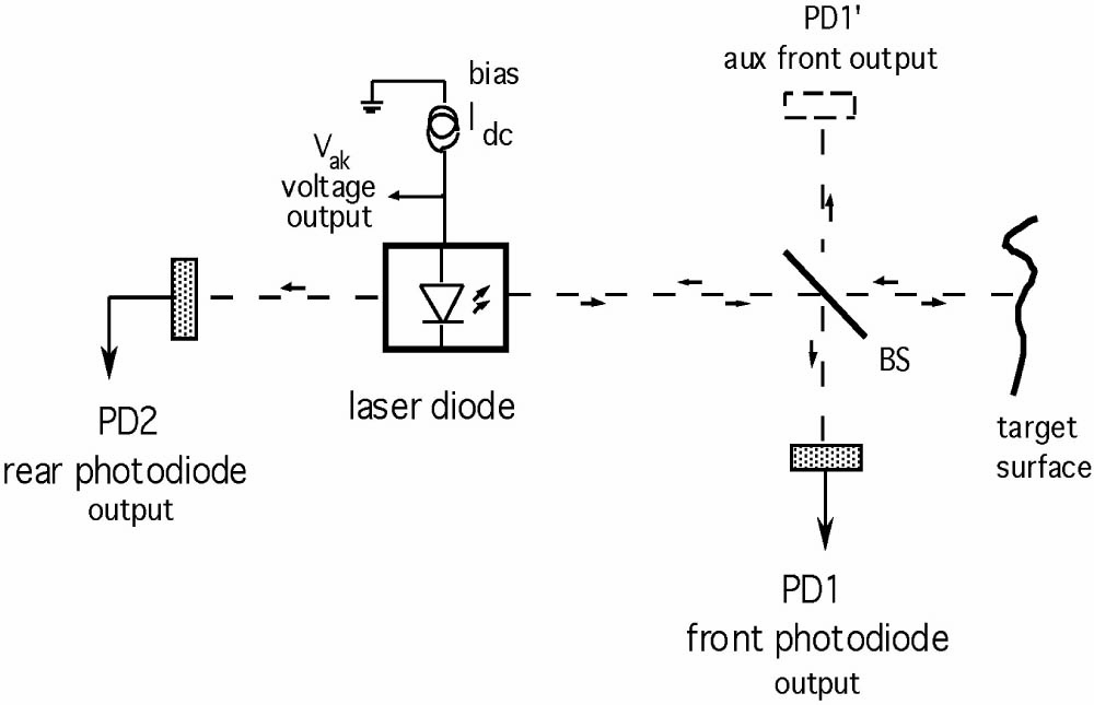
One specific feature of the SMI is that the interferometric signal is carried by the beam. It is found not only on the rear output where the monitor PD2 is placed (see Fig. 1), but also on the front output, where it can be picked up by a beamsplitter (BS) and PD1, as well as on the target itself (not shown in Fig. 1) and on the returning beam by means of PD1′.

Sign up for Chinese Optics Letters TOC. Get the latest issue of Chinese Optics Letters delivered right to you！Sign up now

Figure 1.Different pickups of the output signal from an SMI: from rear PD2 and from front mirrors PD1 and PD1′.

Placing the detecting PD on the target allows us to exploit a unique property of the SMI, namely, measuring the displacement or vibration of a target from the target location itself while it is moving, but this possibility will not be developed in this paper. Another special feature of SMI with a semiconductor laser is the availability of the signal across the anode-cathode terminals of the laser diode (not shown in Fig. 1), which in this case works also as a detector—a feature demonstrated for SMI operation at terahertz (THz) frequency^[4]. More commonly, however the rear PD2 signal is used because it is normally already available in the laser diode package, and it does not obstruct the path of propagation to the remote target.

Also, the placement of the detector on the front beam output is interesting, because the signal here is in phase opposition to that detected at the rear mirror in semiconductor laser diodes driven well above threshold, as found by the analysis presented in Ref. [5].

Therefore, with the difference signal of the two outputs, the amplitude of the SMI signal improves by a factor of two, as experimentally verified in Ref. [6].

Additionally, it is reasonable to expect that the two outputs, which are generated by the same optical field $E_{0}$ traveling back and forth in the laser cavity, are affected by the same noise carried by $E_{0}$ (that is to say, the two output noises are correlated). Thus, the difference signal has less noise than the two SMI signals, or its signal-to-noise ratio (SNR) is further improved.

If this conjecture proves correct, the performance of the SMI is improved in its ultimate sensitivity or detectable noise-equivalent-displacement (NED)^[2].

In this paper, we analyze the noise of the two outputs (front and rear) and their difference with a semiclassical noise model^[7], which accounts for second quantization and find that indeed the two outputs have a partial correlation of noise and that the SNR can be improved up to about 10 dB by the differential signal. Then, we test the theoretical results with a 650 nm laser diode SMI and are able to measure an 8.2 dB improvement of SNR, which is in good agreement with theory.

2. Theoretical Model and Analysis

To avoid unnecessary complications, we consider the simplified scheme of Fig. 2 to evaluate the signal and noise of the front and rear outputs of the laser diode, with the photodetectors placed directly on the outputs of the laser. The power reflectivities of mirrors M1 and M2 are $R_{1}$ and $R_{2}$ , the powers exiting from mirrors are $P_{1}$ and $P_{2}$ , and they are converted into electrical current signals $I_{1} = σ P_{1}$ and $I_{2} = σ P_{2}$ by PD1 and PD2. We suppose that PD2 is totally absorbing and PD1 is partially reflecting, so as to act as the target and generate the feedback field re-entering the laser cavity after propagation to distance $s$ and the accumulated optical phase shift $ϕ = 2 k s$ .

Figure 2.Simplified scheme of an SMI for the evaluation of front and rear output signals and noise.

The output power $P$ is related to the electrical field amplitude $E$ by the well-known Poynting’s relation $P = a E^{2} / {2 Z}_{0}$ , where $a$ is the cross-section area of the beam, and $Z_{0}$ is the vacuum impedance. In the following, however, we write simply $P_{1} = E_{1}^{2}$ and $P_{1} = E_{2}^{2}$ for the powers exiting at mirrors M1 and M2.

Now, we want to calculate the quiescent amplitude of the fields $E_{1}$ and $E_{2}$ as a function of the unperturbed internal field $E_{0}$ and their SMI amplitude variations $Δ E_{1}$ and $Δ E_{2}$ due to a feedback from the target at distance $s$ returning into the cavity with a fraction $A$ of the field $E_{0}$ (taken just before M1, see Fig. 2). The problem was solved in Ref. [5] with the following result for the output field amplitudes $E_{1}$ and $E_{2}$ when perturbed by a small return $A E_{0}$ from the target along a phase shift $ϕ = 2 k s$ : $E_{1} = t_{1} E_{0} {1 - (t_{1}^{2} / r_{1}) (A \cos ϕ) [{(2 γ L + \ln R_{1} R_{2})}^{- 1} - R_{1} / T_{1}]},$ (1) $E_{2} = \sqrt (r_{1} / r_{2}) t_{2} E_{0} [1 - (t_{1}^{2} / r_{1}) (A \cos ϕ) {(2 γ L + \ln R_{1} R_{2})}^{- 1}],$ (2)where $A$ is the attenuation suffered by the field signal on the go-and-return path; $ϕ = 2 k s$ is the optical phase accumulated in the path to the target and back, with $k = 2 π / λ$ the wavevector and $s$ the target distance; $r_{1, 2} = \sqrt R_{1, 2}$ and $t_{1, 2} = \sqrt R = T_{1, 2}$ are the field reflection and transmission of mirrors M1 and M2, respectively; $2 γ L$ is the round-trip gain along the laser cavity of length $L$ ; and factor one in curl parentheses indicates the quiescent (or unperturbed) value of the field, to which the AM term induced by the self-mixing is added.

From Eqs. (1) and (2), we can calculate the modulation indices $m_{1}$ and $m_{2}$ , defined as the ratio of the SMI signal (the term added to unity) and the constant unperturbed field superposed to them, $E_{1, 2}$ for $A = 0$ , and the result is $m_{1} = (t_{1}^{2} / r_{1}) (A \cos ϕ) [{(2 γ L + \ln R_{1} R_{2})}^{- 1} - R_{1} / T_{1}],$ (3) $m_{2} = (t_{1}^{2} / r_{1}) (A \cos ϕ) {(2 γ L + \ln R_{1} R_{2})}^{- 1};$ (4)hence, the ratio $m_{1} / m_{2} = 1 - (R_{1} / T_{1}) (2 γ L + \ln R_{1} R_{2}) .$ (5)

Because of Eq. (5), the outputs are in phase ( $m_{1} / m_{2} = 1$ ) at threshold ( $2 γ L = - \ln R_{1} R_{2}$ ), then, in normal operating conditions above threshold, $2 γ L + \ln R_{1} R_{2} > T_{1} / R_{1}$ , and the outputs become in phase opposition ( $m_{1} / m_{2}$ negative, typically $\approx - 3$ ). The difference in modulation indices of the rear and front outputs is explained by the extra contribution, in the front output, coming from the reflection; on the front mirror, the field returns from the remote target.

In practical operation of a laser diode, the amplitudes of the constant component upon which the SMI is superposed can be brought to the same value, let us say one, by (noiseless) amplification. Then, the SMI signal amplitudes are given just by the modulation indices of Eqs. (3) and (4).

An interesting feature of these dependences is that the difference signal is twice the semi-sum of (absolute) amplitudes as soon as one of the two changes its sign, the case of $m_{1}$ at increasing bias. To see this, let us write Eqs. (3) and (4) in the form: $m_{1}^{'} = g - r$ , and $m_{2}^{'} = g$ . Then, the difference signal is $m_{1}^{'} - m_{2}^{'} = - r$ at all times. But, when $m_{1}^{'}$ changes its sign, its (positive) amplitude is $r - g$ and the semi-sum is $½ (m_{1}^{'} + m_{2}^{'}) = r / 2$ ; accordingly, the ratio $| (m_{1}^{'} - m_{2}^{'}) | / ½ (m_{1}^{'} + m_{2}^{'})$ is equal to two (in absolute value). For clarity, a numerical example about this statement is provided in Appendix A.

In conclusion, although the amplitudes of the SMI output signals and their ratio [Eq. (5)] may change with gain $γ$ —or with bias current—their difference is always double the average (or semi-sum) amplitude of the output signals.

3. Noise Model and Calculations

We model the SMI noise with the scheme of Fig. 3 bottom, which is rigorous from the point of view of second quantization, as described in Ref. [7]. The oscillating field $E_{0}$ is assumed constant in the cavity, and the coherent state fluctuation $Δ E_{coh}$ is attributed to it. The fluctuation $Δ E_{coh}$ is a Gaussian noise of amplitude such that the power $P_{0} = a E_{0}^{2} / 2 Z_{0}$ carried by the field $E_{0}$ has the classical quantum (or shot) noise, $σ_{p}^{2} = 2 h ν P_{0} B$ , where $B$ is the bandwidth of observation^[6]. Explicitly, the fluctuation $Δ E_{coh}$ has zero average, $〈 Δ E_{coh} 〉 = 0$ , and a quadratic mean value given by $〈 Δ E_{coh}^{2} 〉 = (a / 2 Z_{0}) ½ h ν B$ , or, also, a power spectral density $d 〈 Δ E_{coh}^{2} 〉 / d f = ½ h ν$ of a half-photon per hertz. In the following, we omit for simplicity the factor $a / {2 Z}_{0}$ .

Figure 3.Top: the laser diode cavity has mirrors with (power) reflectivity R₁ and R₂, and the optical oscillating field E₀ is assumed constant inside the cavity; bottom: the second-quantization model, in which field E₀ is accompanied by the coherent state fluctuation ΔE_coh, and the vacuum state fluctuations ΔE_vac1,2 enter in the unused port of the mirrors, described as a BS because they have non-unitary transmission.

Additional to the noise carried by the oscillating field, we shall consider also noises entering the unused port of BSs and partially reflecting mirrors. Indeed, for the second quantization, every port left unused is actually a port left open to the vacuum state fluctuation; that is, a field fluctuation, let us call it $Δ E_{vac}$ (see Fig. 3), is equal to the coherent state fluctuation, $Δ E_{vac} = Δ E_{coh}$ , consistent with the fact that the coherent state fluctuation $Δ E_{coh}$ is independent from the value of the field $E_{0}$ and is therefore found also where it is $E_{0} = 0$ , i.e., at unused ports^[7].

With the addition of $Δ E_{vac 1}$ and $Δ E_{vac 2}$ in Fig. 3, the noise model is complete^[7], and we can calculate the fluctuations of output fields $E_{1}$ and $E_{2}$ as well as the variance of noises superposed to output powers $P_{1}$ and $P_{2}$ .

In the classical picture, the output powers $P_{1}$ and $P_{2}$ are affected by the shot noise due to the Poisson distribution of photons that are carried along, and the variance of the power fluctuation is given by the well-known shot-noise expression $σ_{P}^{2} = 2 h ν P B$ . As it is generated by the same power $P_{0}$ traveling back and forth in the cavity, the powers $P_{1}$ and $P_{2}$ have some correlation in their shot-noise fluctuation, but not complete correlation because the mirrors select at random which photon is transmitted and which is reflected.

In the following, we calculate the variances $σ_{P 1}^{2}$ and $σ_{P 2}^{2}$ for the two outputs, as made up by two terms each: one totally correlated and another totally uncorrelated to the corresponding term of the other output, so that the first can be cancelled out in a differential operation, and we can evaluate the SNR improvement thereafter.

With reference to Fig. 3, let us now compute mean value and variance of power delivered at output 1, $P_{1} = 〈 E_{1}^{2} 〉$ (having omitted for simplicity the multiplying term $a / {2 Z}_{0}$ ); also, for simplicity, let us assume equal mirror reflectivity, $R_{1} = R_{2} = R$ . Then, at mirror $M_{1}$ , we can write $E_{1} = t (E_{0} + Δ E_{coh}) + i r Δ E_{vac 1},$ (6)where $t = \sqrt T$ and $r = \sqrt R$ are the field transmission and reflection coefficients of the mirrors, $Δ E_{coh}$ is the Gaussian, zero average, and field fluctuation affecting $E_{0}$ (and independent from amplitude $E_{0}$ ), and $Δ E_{vac 1}$ is the same distribution, but uncorrelated to $Δ E_{coh}$ , which enters as the vacuum fluctuation^[7] from the unused port of the BS. The properties are $〈 Δ E_{coh} 〉 = 〈 Δ E_{vac 1} 〉 = 0, and σ_{E}^{2} = 〈 Δ E_{coh}^{2} 〉 = 〈 Δ E_{vac 1}^{2} 〉 = ½ h ν B .$ (7)

Now, the mean value of $P_{1}$ is given by the classical expression $P_{1} \propto E^{2}$ but subtracted from the square average of the vacuum field (because this cannot be observed)^[7]: $P_{1} = 〈 | E_{1}^{2} | 〉 - 〈 Δ E_{vac 1}^{2} 〉 .$ (8)

Inserting Eq. (6) into Eq. (8) we get $P_{1} = t^{2} E_{0}^{2} + t^{2} 〈 Δ E_{coh}^{2} 〉 + r^{2} 〈 Δ E_{vac 1}^{2} 〉 + {2 t}^{2} 〈 E_{0} E_{coh}^{2} 〉 + 2 t r 〈 E_{0} E_{vac 1} 〉 + 2 t r 〈 E_{coh} E_{vac 1} 〉 - 〈 Δ E_{vac 1}^{2} 〉,$ (9)and, because the second, third, seventh, and the last terms on the right-hand side cancel out, we get $〈 P_{1} 〉 = t^{2} E_{0}^{2} + 2 t^{2} 〈 E_{0} E_{coh} 〉 + 2 t r 〈 E_{0} E_{vac 1} 〉 + 2 t r 〈 E_{coh} E_{vac 1} 〉 .$

As the mean value of $E_{coh}$ and $E_{vac 1}$ is zero, $E_{coh}$ and $E_{vac 1}$ are uncorrelated, and, noting that $E_{0}^{2} = P_{0}$ and $t^{2} = T$ , we get $〈 P_{1} 〉 = t^{2} E_{0}^{2} = T P_{0},$ (10)i.e., just the expected result.

Variance is calculated as the difference $σ_{P 1}^{2} = 〈 P_{1}^{2} 〉 - 〈 P_{1} 〉^{2}$ , or $σ_{P 1}^{2} = t^{4} E_{0}^{4} + 4 t^{2} 〈 E_{0}^{2} E_{coh}^{2} 〉 + 4 t^{2} r^{2} 〈 E_{0}^{2} E_{vac 1}^{2} 〉 - t^{4} E_{0}^{4}$ + vanishing double products.

Substituting $t^{2} = T$ and $r^{2} = R$ , we get $σ_{P 1}^{2} = 4 T^{2} E_{0}^{2} 〈 E_{coh}^{2} 〉 + 4 T R E_{0}^{2} 〈 E_{vac 1}^{2} 〉,$ (11)and, using $T E_{0}^{2} = P_{1}$ and $〈 E_{coh}^{2} 〉 = 〈 E_{vac 1}^{2} 〉 = ½ h ν B$ , we finally obtain $σ_{P 1}^{2} = 2 T P_{1} h ν B + 2 R P_{1} h ν B .$ (12)

Worth noting, as $R + T = 1$ , Eq. (12) is also written as $σ_{P 1}^{2} = {2 P}_{1} h ν B$ , that is, the classical variance expected for a Poisson-statistics power $P_{1}$ .

Now, we can repeat the calculation for exit 2, and it is straightforward to write the result as $P_{2} = P_{1}, σ_{P 2}^{2} = 4 T^{2} E_{0}^{2} 〈 E_{coh}^{2} 〉 + 4 T R E_{0}^{2} 〈 E_{vac 2}^{2} 〉 = 2 T P_{2} h ν B + 2 R P_{2} h ν B .$ (13)

Note that the first right-hand side terms of Eqs. (12) and (13) are the same as those derived from the same process, the beating of signal with its coherent state fluctuation, so they are completely correlated and will be canceled out, making the difference $P = P_{1} - P_{2}$ . Instead, the second right-hand side terms of Eqs. (12) and (13) are completely uncorrelated because they come from different independent fluctuations, $E_{vac 1}$ and $E_{vac 2}$ .

Taking account of the correlations, we get the variance of $P = P_{1} - P_{2}$ , $σ_{P 2 - P 1}^{2} = 4 T R E_{0}^{2} 〈 E_{vac 1}^{2} 〉 + 4 T R E_{0}^{2} 〈 E_{vac 2}^{2} 〉 = 8 T R P_{0} ½ h ν B = 4 R P_{1} h ν B$ (14)to be compared to $σ_{P 1}^{2} = σ_{P 2}^{2} = 2 P_{1} h ν B$ . Therefore, the ratio of free and differential variance is $σ_{P 2 - P 1}^{2} / σ_{P 1}^{2} = 2 R,$ (15)and the corresponding SNR, considering the doubling of the differential signal becomes $F = {({SNR}_{P 2 - P 1} / {SNR}_{P 1})}^{2} = (4 / 2 R) / 1 = 2 / R .$ (16)

For a semiconductor laser with a typical $R = 0.3$ , we get $F = 2 / 0.3 = 6.6 (or 8.2 dB) .$

About the output voltage signal $V = R_{t r} σ P$ obtained across a resistance $R$ fed by the PD current $I = σ P$ , we have for the SNR the same ratio, or ${({SNR}_{P 2 - P 1} {/ SNR}_{P 1})}^{2} = {({SNR}_{V 2 - V 1} / {SNR}_{V 1})}^{2} or also {SNR}_{V 2 - V 1} / {SNR}_{V 1} = \sqrt F, and 20 \log \sqrt F = 10 \log F = 8.2 dB .$

For a He–Ne laser, the front and rear outputs are in phase, in the normal operation of the source^[5], so the factor two of the differential outputs is not achieved, and we have $F = 1 / R$ . Moreover, as the reflection coefficient of typical He–Ne mirrors is $R = 0.95 - 0.98$ , the improvement in $F$ is marginal.

With a slightly different method based on second quantization, Elsasser and coworkers^[8] have calculated the correlations of the output fields in a Fabry–Perot laser, including the effects of internal absorption and spatial hole burning, with the aim of generating correlated light beams, and found correlation factors up to 0.8. The low-frequency suppression of $1 / f$ components in a laser diode by output subtraction has been investigated by Fronen^[9] finding almost complete correlation between the two outputs.

3.1. Extension of the noise results

Usually, Fabry–Perot semiconductor lasers have cleaved facets, so $R_{1} = R_{2}$ and the results of previous sections apply. However, one can come across lasers with $R_{1} \neq R_{2}$ , and, therefore, we extend the theory to the general case of different mirror reflectivity.

By repeating the calculations of previous sections, we find that, upon equalizing the output power amplitudes, the variance of the output difference is given by $σ_{P 2 - P 1}^{2} = 2 (R_{2} T_{1} + R_{1} T_{2}) \sqrt (R_{1} R_{2}) P_{00} h v B,$ where $P_{00}$ is the power at the crossover point internal to the laser, at which left-going and right-going beams are of equal power. Moreover, the variances of the outputs—after balancing the mean power signal—are $σ_{P 1 or 2}^{2} = 2 \sqrt (T_{1} T_{2}) \sqrt (R_{1} R_{2}) P_{00} h ν B;$ hence, the variance ratio becomes $σ_{P 2 - P 1}^{2} / s_{P 1 or 2}^{2} = (R_{2} T_{1} + R_{1} T_{2}) / \sqrt T_{1} T_{2},$ (17)for $R_{2} = R_{1} = R$ , and $T_{1} = T_{2} = T$ , and Eq. (17) gives the same as Eq. (15). Also, the improvement in SNR is given by $F = 2 \sqrt (T_{1} T_{2}) / (R_{2} T_{1} + R_{1} T_{2})$ , which becomes $F = 1 / 2 R$ for equal $R$ and $T$ .

3.2. Picking the front output signal

As mentioned above, the receiving PD placed on the front output of mirror M1 can also serve, with its transparent window reflecting a few percent of the incoming radiation, as the target surface while intercepting practically all of the power $P_{1}$ available. However, when this arrangement is not allowed by the application, normally because of its invasiveness, we can use either a BS, deviating a fraction of the power in transit to the P1, as shown in Fig. 4 (top), or a partial removal of the outgoing beam (see below).

$(top) Pickup of the front SMI signal by means of a BS, deviating a fraction RBS of power P1 to PD1; (bottom) equivalent circuit for the evaluation of noise, showing the added fluctuation ΔEvacBS entering in the unused port of the BS.$

Figure 4.(top) Pickup of the front SMI signal by means of a BS, deviating a fraction R_BS of power P₁ to PD1; (bottom) equivalent circuit for the evaluation of noise, showing the added fluctuation ΔE_vacBS entering in the unused port of the BS.

The BS offers a compact solution to power pickup, because it may be as small as the beam, but has the serious disadvantage of opening a port to the vacuum fluctuation, term $Δ E_{vac B S}$ in Fig. 4 (bottom).

The calculation of powers and associated variances follows the guidelines of previous sections, and, for brevity, we will omit here the detailed development of the analysis, limiting ourselves to report the results. For $R_{1} = R_{2} = R$ , it is found that the power at the detector PD1 is given by $P_{1 B S} = {(r_{B S} t)}^{2} E_{0}^{2} = R_{B S} P_{1} = T R_{B S} P_{0},$ (18)while the power at the other mirror is still $P_{1} = t^{2} E_{0}^{2} = T P_{0}$ , larger than $P_{1 B S}$ , and this circumstance will generally require a balance operation to get equal amplitude levels. The variance of fluctuations associated with $P_{1 B S}$ is $σ_{P 1 B S}^{2} = 2 T R_{B S} P_{1 B S} h ν B + 2 (R R_{B S} + T_{B S}) P_{1 B S} h ν B = 2 T R_{B S}^{2} P_{1} h ν B + 2 R_{B S} (R R_{B S} + T_{B S}) P_{1} h ν B .$ (19)

After the (noiseless) power amplification by factor ${1 / R}_{B S}$ to equalize the amplitude of $P_{1 B S}$ before subtracting $P_{2}$ , so that we obtain $P_{1} - P_{2} = {2 P}_{1}$ , we get the equalized variance $σ_{P 1 B S (eq)}$ : $σ_{P 1 B S (eq)}^{2} = σ_{P 1 B S}^{2} / R_{B S}^{2} = [2 T R_{B S}^{2} P_{1} h ν B + 2 R_{B S} (R R_{B S} + T_{B S}) P_{1} h ν B] / R_{B S}^{2} = 2 T P_{1} h ν B + 2 (R + T_{B S} / R_{B S}) P_{1} h ν B$ (20)to be compared with $σ_{P 1}^{2} = 2 T P_{1} h ν B + 2 R P_{1} h ν B,$ where the first terms (correlated) cancel out again, and the second terms give the difference as $σ_{P 2 - P 1}^{2} = 2 (2 R + T_{B S} / R_{B S}) P_{1} h ν B, and {SNR}_{P 1 - P 2}^{2} = [4 / 2 (2 R + T_{B S} / R_{B S})] (P_{1} h ν B) = [2 / (2 R + T_{B S} / R_{B S})] (P_{1} h ν B)$ (21)to be compared to the single-channel ${SNR}_{P 1}^{2} = P_{1} / 2 h ν B$ , where the final result $F = {({SNR}_{P 2 - P 1} / {SNR}_{P 1})}^{2} = 2 / (R + T_{B S} / 2 R_{B S}) .$ (22)

From Eq. (22), we can see that the BS affects severely the improvement factor $F$ . Indeed, if we chose a $50 / 50 B S$ , $F$ would be less than two. For the improvement to be comparable to $F = 2 / R$ of the direct configuration (Fig. 2), we shall limit $T_{B S} / {2 R}_{B S}$ to a fraction of $R$ ; for example, taking $T_{B S} = 0.05$ to have $F = 7.8 dB$ , or $T_{B S} = 0.10$ for $F = 7.5 dB$ . At these low values of transmittance, almost all of the power of the M1 output is taken by the PD, and only a small fraction of $T_{B S}$ is used to sense the remote target. As a consequence, the SMI signal is decreased, and the performance is worsened, so that the improvement of $F$ of the differential output becomes illusory.

The second method, consisting of sampling the outgoing beam by removing a small portion of it by means of a totally reflecting prism (or a mirror) is depicted in Fig. 5.

Figure 5.Portion a′ of the beam outgoing from mirror M1 by means of a reflecting prism.

The power collected by this arrangement is the ratio of areas $a^{'}$ and $a + a^{'}$ of the intercepted beam and the total beam, or $P_{1 P} = [a^{'} / (a + a^{'})] P_{1}$ (Fig. 5). However, at equal $a^{'} / (a + a^{'})$ and $R_{B S}$ , the fractional pickup of the beam is dramatically different from the BS pickup, because it does not open the port to the vacuum fluctuations (as the BS in Fig. 4 does). This is due to the total reflection of the prism (or of a mirror in place of it) that makes the arrangement a two-port device instead of the four ports of the BS (Fig. 4).

Therefore, for this configuration, the expressions of variance [Eqs. (12) and (13)] hold with $P_{1}$ replaced by $P_{1 P}$ , and the variance ratio of the signal difference [Eq. (14)] and the improvement [Eqs. (15) and (16)] also apply.

4. Experimental Validation

We carried out the experiment with a 650 nm diode laser, Roithner QL65D6SA with a Fabry–Perot structure. The laser had a threshold of 30 mA and was biased at 40 mA and emitted at 5 mW. The monitor PD incorporated in the package supplied a 0.2 mA current, so it was receiving only about 10% of the power emitted by the rear mirror. This simplified the balancing operation with the $10 % = a^{'} / (a + a^{'})$ power picked up by a 3.1 mm side rectangular prism on the beam of about $w_{0} = 10 mm$ at the exit of an $F = 5 mm$ , $NA = 0.53$ collimating lens. PD1 was fed to a transimpedance amplifier with $R_{f 1} = 4.7 kΩ$ feedback resistance and PD2 to another transimpedance amplifier feedback resistance $R_{f 2}$ adjustable between 1 and 10 kΩ. A difference operational amplifier provided a signal proportional to $P_{P 1} - P_{2}$ , and its output was directly sent to a digital oscilloscope. The target was a loudspeaker placed at 10 cm distance, with the central part covered by plain white paper. To balance the two channels, we applied a 1.5 mA triangular waveform to the bias current and adjusted $R_{f 2}$ so as to reach the condition of equal amplitude, or near to zero difference, as shown in Fig. 6.

Figure 6.Balancing of the two SMI signals detected by PD1 and PD2: a triangular waveform is applied to the bias and generates detected responses brought to be nearly identical (top trace), that is, with a residually small difference (bottom trace).

Then, we analyze the difference signal $P_{P 1} - P_{2}$ and its fluctuations, both in the frequency domain by means of a spectrum analyzer and as a total amplitude by means of an ac-coupled rms voltmeter.

In Fig. 7, we report the result of spectral noise measurement of the two channels $P_{P 1}$ and $P_{2}$ , and of their differential fluctuation, which is 2.5 dB smaller. Taking account of the doubling of signals [which amounts to 6 dB for their square, see Eq. (22)], the SNR improvement is $2.5 + 6 = 8.5 \pm 1 dB$ .

Figure 7.Signals detected by PD1 and PD2 (red and blue) and their difference (yellow), exhibiting a noise 2.5 ± 1 dB smaller.

We have also measured the total amplitude fluctuations of the two channels and of their difference and found that the improvement is even better than that recorded by the spectral density, typically of 2–3 dB. This is due to the presence, on both channels, of electrical disturbance (i.e., electromagnetic interference, EMI) and the $1 / f$ noise component collected almost equally by both channels and obviously cancelled by the difference operation. For example, in Fig. 8, we report an example of the SMI channels deliberately disturbed by an EMI perturbation generated by the brushes of an electrical motor placed in close proximity to the optical SMI. The series of peaks at frequencies from 30 to 300 kHz are reduced in amplitude by about 25 to 30 dB thanks to the difference operation.

Figure 8.Peaks of EMI superposed to the SMI of channels PD1and PD2 (yellow and yellow–green) and the difference channel (red), exhibiting a disturbance reduction of 25…30 dB.

5. Conclusions

We have demonstrated that the difference signal of the two outputs—front and rear—of a laser diode SMI has an improved SNR with respect to each of the two outputs. On a Fabry–Perot laser, we have measured an improvement of $8.5 \pm 1 dB$ , which is in good agreement with the theoretical value of 8.2 dB. We have also found that EMI collected by the two channels is strongly reduced (of 25–30 dB) by the difference operation. The improvement is due to the two signals being in phase opposition above the threshold and to the partial correlation of the noises as shown by an analysis based on a second-quantization model.

References

[1] S. Donati. Developing self-mixing interferometry for instrumentation and measurements. Laser Photon. Rev., 6, 393(2012).

[2] S. Donati. Electro-Optical Instrumentation–Sensing and Measuring with Lasers(2004).

[3] S. Donati, M. Norgia. Overview of self-mixing interferometer applications to mechanical engineering. Opt. Eng., 57, 051506(2018).

[4] P. Dean, Y. L. Lim, A. Valavanis, R. Kleise, M. Nikolic, D. Indjin, Z. Ikonic, P. Harrison, A. D. Rakic, E. H. Lindfield, G. Davies. Terahertz imaging through self-mixing in a quantum cascade laser. Opt. Lett., 36, 2587(2011).

[5] E. Randone, S. Donati. Self-mixing interferometer: analysis of the output signals. Opt. Express, 14, 9788(2006).

[6] K. Li, F. Cavedo, A. Pesatori, C. Zhao, M. Norgia. Balanced detection for self-mixing interferometry. Opt. Lett., 42, 283(2017).

[7] S. Donati. Photodetectors–Devices, Circuits and Applications, 427(2021).

[8] J. L. Vey, K. Auen, W. Elsasser. Intensity fluctuation correlations for a Fabry–Perot semiconductor laser: a semiclassical analysis. Opt. Commun., 146, 325(1998).

[9] R. J. Fronen. Correlation between 1/f fluctuations in the two output beams of a laser diode. J. Quantum. Electron., 27, 931(1991).