Shaping and tailoring distribution of amplitude, phase, and polarization of light has become a subject of rapidly growing interest, due to its unique properties and novel applications in various scientific and engineering realms, such as optics trapping^[1,2], surface plasma excitations^[3], super-resolution^[4], and laser micromachining^[5]. Besides, it has been proved that light beams with a polarization gradient, aiming at exploiting the vectorial nature of the light, can exert forces and torques on the illuminated particle for special purposes^[6–9]. These demands in optical science prompt the everlasting quest to find novel methods of completely controlling the structure of light fields^[10,11].

Currently, several methods, based on the superposition of orthogonal base vector components and a computer-generated hologram (CGH) on the spatial light modulator (SLM), have been proposed to create and shape the desired vector field^[12–18], including iterative^[12] and non-iterative methods^[13–18]. However, the vector fields as mentioned above have a common feature in that the amplitude of the base vector is uniform so that the state of polarization (SoP) of the synthesized vector beam varies only along a equator circle^[15–17] or prime meridian circle^[18] on the Poincaré sphere (PS), wherein two quarter-wave plates (QWPs) and two half-wave plates (HWPs) are employed, respectively, but unable to span the entire surface of the PS. Generally, the construction of genuine Poincaré vector beams (PVBs) needs four independent modulation degrees of freedom, one for the amplitude, one for phase retardation, and two for the polarization^[14,19], which is not a trivial task and requires a deliberate design.

In this Letter, we extend a scheme reported in Ref. [20] for creating scalar beams to synthesize vector beams and propose to produce in the far field (viz., the focal field of focusing lenses) a new kind of PVBs that are curved in the three-dimensional (3D) space, termed curvilinear PVBs (CPVBs). We design CPVBs based on the superposition of two orthogonally polarized beams^[21], both of which possess the same curve locus but an independently prescribed amplitude and phase distribution, and demonstrate experimentally that the created CPVBs contain arbitrarily tailorable amplitude, phase, as well as polarization gradients with high intensity gradients prescribed along any 3D trajectories. Furthermore, the 3D curve rendered by the CPVB can be mapped onto a continuous curve on the PS surface.

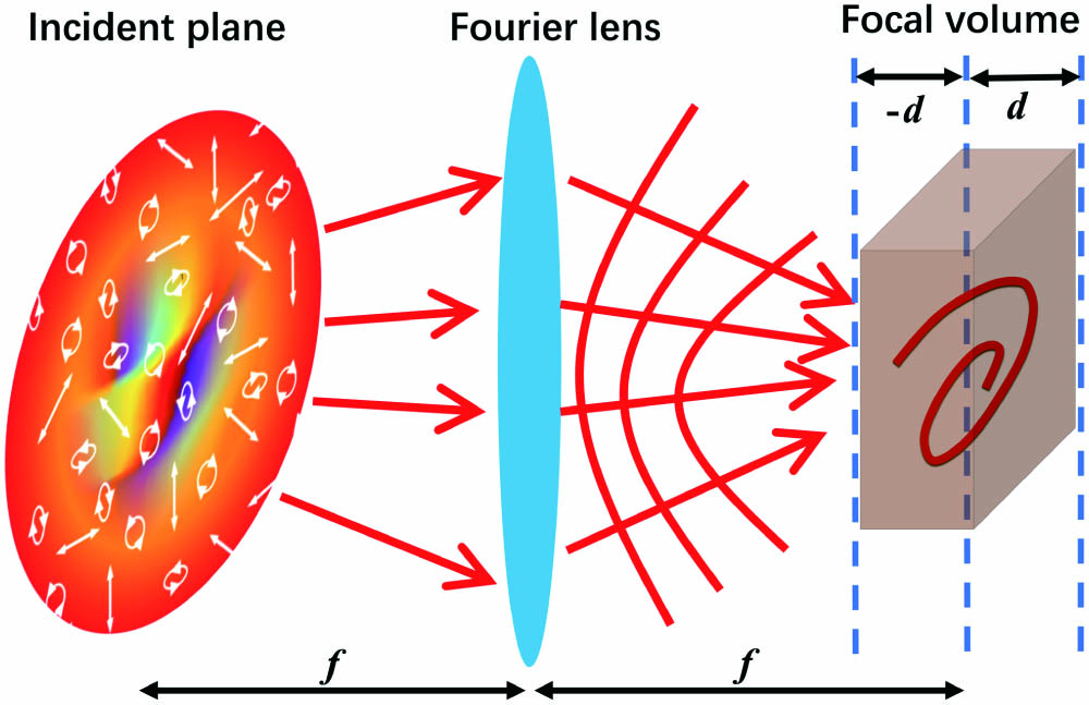
Let us consider a focusing process under the paraxial condition, as shown in Fig. 1. We want to generate a desired focal beam that can trace out a 3D curve represented by Cartesian coordinate [x0(t),y0(t), z0(t)] with the azimuthal angle t∈[0,T], where T stands for the maximum value of the azimuthal angle. For this purpose, we need to design a complex amplitude of the incident light field given by the following expression: H(x,y)=∫0Tg(t)ψ(x,y,t)φ(x,y,t)dt.(1)

The terms g(t), ψ(x,y,t), and φ(x,y,t) in Eq. (1) are determined by^[20]{g(t)=α(t)exp[iϕ(t)]x0′(t)2+y0′(t)2+z0′(t)2,ψ(x,y,t)=exp{−iw02[xy0(t)+yx0(t)]},φ(x,y,t)=exp[iπx2+y2λf2z0(t)],(2)where w0 is a constant. The term x0′(t)2+y0′(t)2+z0′(t)2 in Eq. (2) guarantees a uniformly distributed intensity along the curve, while α(t) acts as a free parameter for controlling the variation gradient of amplitude along the curve. ϕ(t) is a phase function that dominates the phase gradient along the curve. Dynamic modulation of amplitude along the curve can be acquired by changing the dependence of α(t) on the parameter t in a certain way. The term ψ(x,y,t) controls the position of each focused spot in the focal plane, while the term φ(x,y,t) controls the focusing distance through a quadratic phase function, wherein f and λ represent the focal length of the Fourier lens and the wavelength, respectively.

Equation (1) allows us to calculate the incident complex field that can shape a structurally stable scalar focal beam with prescribed arbitrary amplitude and phase gradient along a curve in the focal volume of the lens. First, we consider the generation of an Archimedean curve represented by x0(t)=−R0tcos(10t), y0(t)=−R0tsin(10t), and z0(t)=sR0[0.5−(1−t2)1/2], with t∈[0,1] and s=0 for a two-dimensional (2D) or else a 3D curve, with different amplitude and phase gradient, and show by simulation the controlling capability of amplitude and phase. As an illustration, Fig. 2 shows the simulated results (R0=0.275mm), where the left and right halves of Fig. 2 display the amplitude and phase distribution of the resulting beams, respectively; the sub-graphs with labels (ai) and (bi) with i(=1,2,…,6) represent the amplitude and phase of the ith beam, respectively. The first row in Fig. 2 presents the uniform amplitude distribution, while the second shows the ability to control arbitrary amplitude variations along the curve by adjusting the amplitude distribution terms in Eq. (2) such as α(t)=|sin(2πt)|. Note that the amplitude distribution through rows 1 to 2 is different, while the phase through rows 1 to 2 has the same structure. Therefore, it shows that the amplitude gradient α(t) and phase gradient ϕ(t) are independently controlled. The 3D structure of controllable amplitude Archimedean curve is revealed along the beam propagation in the focal region in simulation, as shown in Figs. 2(c) and 2(d), respectively. The beam intensity distributions calculated at the focal plane (z=−25,−15,−5,0, and 15 mm, respectively) are shown in Figs. 2(e) and 2(f). It should also be noted that the term ϕ(t)=2πm∫0tdl/∫0Tdl actually resembles the phase ramp of perfect optical vortices^[15] with an index m that denotes the topological charge of the vortex and is independent of the size of the curve beam, as shown in Fig. 2.

We now consider the realization of a CPVB. As is well-known, any SoP can be geometrically represented by a point on the PS surface through the spherical coordinate (2χ, 2ϕ) as follows^[22]: $$\begin{gathered} p^(2χ,2ϕ)=sin(χ+π4)exp(−jϕ)e^r \\ +cos(χ+π4)exp(jϕ)e^l, \end{gathered}$$(3)where χ and ϕ are also responsible for the ellipticity and angle of the polarization ellipse, respectively. e^r and e^l refer to the right- and left-circular polarization base vector, corresponding to the north and south poles of the PS, respectively. Our proposed CPVB aims to enable the Cartesian coordinates of the beam location [x0(t), y0(t), and z0(t)] to be mapped onto the spherical coordinates (2χ, 2ϕ) on the PS surface by the following relation: {x0(t)=S1=S0cos2χcos2ϕ,y0(t)=S2=S0cos2χsin2ϕz0(t)=S3=S0sin2χ,,(4)where (S0, S1, S2, S3) represent the Stokes parameters constructing the PS and S0=x02+y02+z02. Obviously, given a beam location [x0(t),y0(t), and z0(t)] determined by the spherical coordinates (2χ, 2ϕ), we can calculate the parameters expressed by Eq. (2) and finally find the input light field needed for yielding a desired CPVB. It should be noted that the reason we choose such a beam whose trajectory is reflected on the PS surface is just to give an example for proving the effectiveness of our method; in fact, we can generate any on-demand polarization gradient curve beams, for example, a vector counterpart of the scalar Archimedean-curved beams.

To create the proposed CPVB, we use the aforementioned technique to shape the two scalar 3D curves that have the same path but different phase and amplitude and mutually orthogonal SoPs, and then we employ vector optical field generation techniques to create the CPVB. The experimental setup of the CPVB generation system is schematically illustrated in Fig. 3, which is composed of two parts—one is a vector field generator, and the other is the focusing part for yielding the far field. The detailed working principle can be found in Ref. [15] and is briefly outlined here. First, two complex amplitude fields at the incident plane, denoted as H1(x,y) and H2(x,y), are calculated through Eq. (1) from two constituent beams representing polarization components. Subsequently, each complex amplitude field is imposed by linear phase factors of exp(i2πxsinθx/λ) and exp(i2πysinθy/λ), respectively, and is converted into mutually orthogonal left- and right-circular SoPs using two QWPs in the two optical channels of the filter plane, which serve as a pair of base vector beams for the subsequent vectorial superposition. A Ronchi grating placed at the rear focal plane of the second lens re-corrects the diffraction direction of each beam, enabling the collinear recombination of the two base vector beams. Thus, the holographic function needed to be encoded on the SLM is calculated by $$\begin{gathered} H(x,y)=H1(x,y)exp(i2πxsinθx/λ) \\ +H2(x,y)exp(i2πxsinθy/λ). \end{gathered}$$(5)

The above complex holographic function is encoded into a phase-only CGH by using the cosine-grating encoding method^[23] and imprinted on the phase-only SLM (HOLOEYE Leto, 6.4 µm pixel pitch, 1920×1080). Once the synthesized vector field is input into the focusing system, the 3D CPVB is produced in the focal volume.

We place a polarization camera (4D TECHNOLOGY Polar-Cam G5, 3.45 µm pixel pitch, 2464×2056) in the focal region of the focusing lens (f=100mm) to capture the focused field resulting from the synthesized field H1(x,y)e^r+H2(x,y)e^l. The polarization camera is composed of an array of super-pixels, each of which has four sensor pixels covered by their corresponding micropolarizers with four discrete polarizations (0, 45, 90, 135 deg). Combined with a QWP, the polarization camera can measure the four parameters (S0, S1, S2, S3) simultaneously. By moving the camera back and forth along the optical axis to record the intensity distribution of focal volume, we can accomplish the 3D polarimetric tomography for the focal field and thus reconstruct the 3D trajectory of CPVB.

We now construct ring-shaped CPVBs in the 3D space for demonstration purposes. Assuming that the unit normal vector n^ of the plane occupied by the 3D ring is defined as n^=[nx,ny,nz]T with T representing the transpose of matrix, and letting u^ and v^ stand for two orthogonal unit vectors in the ring plane, (u^,v^,n^) forms the right-hand triplet. In this way, the parameter equation of the 3D ring is defined as [x0,y0,z0]T=R0cos(t)u^+R0sin(t)v^. The projection of the 3D ring onto the x–y plane (i.e., the focal plane) is easily determined by the normal vector of the 3D ring.

Before presenting results of the designed CPVBs, we should address an important aspect associated with the scaling factor in the transverse and longitudinal coordinates of the focal space. Note that the paraxial propagation is assumed in the focusing process, which is a prerequisite of our design method. The paraxial propagation means that the light beam mainly propagates along the z direction. In order to obey this paraxial condition, we specify the trajectory space of the designed beam as [−0.3mm, 0.3 mm] in the transverse dimension and [−8.0mm, 8.0 mm] in the longitudinal dimension, which is assumed in the 3D geometrical drawing of the examples presented in the following context.

Let us present the first CPVB example that represents a common ring in the focal plane by setting n→=[0,cos(π/2),sin(π/2)]T and R0=0.275mm. Correspondingly, this ring-shaped PVB has a space-variant SoP distribution that spans across the equator of the PS, as marked by the black solid circle in Fig. 4(a). The right-circular polarization component field in the input plane is shown in Fig. 4(b), wherein the normalized amplitude (∈[0,1]) and phase (∈[0,2π]) are visualized by the colormap. By moving the polarization camera in the z direction, we measure 101 cross-sectional distributions of the focused field within the range of z∈[−d,d] with d=8.0mm, each of which contains four sets of data used to calculate the Stokes parameters (S0, S1, S2, S3). Figure 4(c) shows the experimentally measured intensity (S0) distributions of the generated CPVB in successive planes at z=−5.6, 0, and 5.6 mm, respectively. For comparison, Figs. 4(d) and 4(e) give the simulation and experimental results of the four Stokes parameters (S0, S1, S2, S3) in the focal plane (z=0), which are shown in order from top to bottom. The experimental results shown in Fig. 4 agree well with the simulation, and the SoP distribution is correctly arranged along the beam’s trajectory. For example, the values of S1 and S2 vary azimuthally, while the value of S3 is almost zero, as shown in Fig. 4(e), indicating the generated beam has azimuthal-variant linear polarization along the ring trace.

We now describe the second example of n→=[0,cos(π/4),sin(π/4)]T, which can be understood as a tilted ring that results from a 45 deg rotation of the ring in the first example around the x axis in the rescaled cubic space, as shown in Fig. 5. Besides tracing out a 3D ring-shaped trajectory, this beam contains hybrid SoPs spanning across the northern and southern hemispheres of the PS, in contrast with the first example, which is comprised of locally linear SoPs only occupying the equator of the PS. Figure 5(b) shows the complex field of one component (right-circular polarization) in the input plane, and Fig. 5(c) presents the experimentally measured intensity of the generated CPVB in the planes at z=−5.6, 0, and 5.6 mm in the focal space, respectively. It can be clearly seen that due to the inclination the beam trajectory appears with a fade-in and fade-out in the successive scenes. The 3D trajectory can also be visualized by the intensity (S0) distribution of the beam in the focal space, shown in Figs. 5(d1) (simulation) and 5(e1) (experiment). It can be seen that the beam intensity is uniformly distributed along the inclined ring in the real space, which is exactly what we expected. The measured Stokes parameters shown in Fig. 5(e), agreeing well with the numerical simulation shown in Fig. 5(d), show that the realized CPVB is indeed endowed with the desired SoPs.

Finally, we explore the simultaneous generation of double CPVBs that trace out two crossed rings in the focal space. The two rings are symmetrically inclined around the z axis by setting n→=[0,cos(π/4),sin(π/4)]T and [0,cos(3π/4),sin(3π/4)]T, respectively, as schematically illustrated in Fig. 6. The presented results show that this double-ring-shaped PVB is constructed as expected, as shown by the simulation in Fig. 6(d), and is satisfactorily realized by the experiment, as shown by the volumetric reconstruction in Fig. 6(e).

In summary, we develop a method for enabling the complete control of amplitude gradients as well as the phase gradient distribution along the 3D trajectory of the light beam, and apply it for generating curvilinear vector beams with prescribed intensity distribution and SoPs. The real-space trajectory of the generated CPVB is endowed with SoPs specified by the analogous trajectory of the Poincaré space. The experimental results demonstrate that the generated CPVBs exhibit high intensity gradients and accurate SoPs prescribed along arbitrary 3D trajectories. Owing to the high intensity gradient and the controllable polarization gradient, the proposed CPVB can provide an optical guiding channel for trapping and moving microscopic particles. Our approach can facilitate exploration and application of the freestyle 3D vector optical manipulation.

References

[9] W. Liu, D. Dong, H. Yang, Q. Gong, K. Shi. Robust and high-speed rotation control in optical tweezers by using polarization synthesis based on heterodyne interference. Opto-Electron. Adv., 3, 200022(2020).
[10] L. Zhang, F. Lin, X. Qiu, L. Chen. Full vectorial feature of second-harmonic generation with full Poincaré beams. Chin. Opt. Lett., 17, 091901(2019).
[18] J. A. Rodrigo, T. Alieva. Vector polymorphic beam. Sci. Rep., 8, 7698(2018).
[19] A. M. Beckley, T. G. Brown, M. A. Alonso. Full Poincare beams. Opt. Express, 18, 10777(2010).
Set citation alerts for the article
Please enter your email address
© Copyright 2018-2021 | Chinese Laser Press. All Rights Reserved 沪ICP备15018463号-20