Measuring the topological charge of optical vortices with a single plate

Jingyin Zhao; Yunxia Jin; Fanyu Kong; Dongbing He; Hongchao Cao; Wang Hao; Yubo Wu; Jianda Shao

doi:10.3788/COL202220.110501

Abstract

Measuring the topological charge (TC) of optical vortex beams by the edge-diffraction pattern of a single plate is proposed and demonstrated. The diffraction fringes can keep well discernible in a wide three-dimensional range in this method. The redundant fringes of the diffracted fork-shaped pattern in the near-field can determine the TC value, and the orientation of the fork tells the handedness of the vortex. The plate can be opaque or translucent, and the requirement of the translucent plate for TC measurement is analyzed. Measurement of TCs up to

\pm 40

is experimentally demonstrated by subtracting the upper and lower fringe numbers with respect to the center of the light. The plate is easy to get, and this feasible measurement can bring great convenience and efficiency for researchers.

Keywords

optical vortex orbital angular momentum topological charge measurement

1. Introduction

In 1992, Allen et al. firstly, to the best of our knowledge, demonstrated a helical phase structure of light with wavefront singularities carrying orbital angular momentum (OAM)^[1]. Such optical vortex (OV) beams characterized by the phase factor $\exp (i l θ)$ , where $l$ donates the OAM state or the topological charge (TC), and $θ$ is the azimuthal angle, have been widely applied in various areas, including optical tweezers^[2], optical trapping^[3], optical communication^[4], and quantum information technology^[5]. Most of these applications require a specific TC. As a consequence, the determination of TCs is of crucial importance.

Many methods are proposed to measure the TC of vortex beams, which can be basically divided into three techniques: interferometry, intensity analysis of OV beams, and diffractometry. Nevertheless, the first technique demands cumbersome interferometric setups and finely aligned optical elements^[6–11]. The intensity analysis of the OV beam with complex algorithms^[12] is not intuitive enough to determine the TC. The present diffractometric methods usually transform OVs into identifiable patterns by specialized components such as apertures^[13–15], lenses^[16,17], and special gratings based on the mode conversion from Laguerre–Gaussian (LG) beams to near Hermite–Gaussian with phase-loaded spatial light modulators (SLMs)^[18–21].

Since the edge diffraction of OV beams was firstly investigated and demonstrated in 1998^[22], to the best of our knowledge, increasing works have revealed its propagation properties due to the helical phase of the OV beam^[23–28]. Masajda et al. showed that the OV beam is capable of self-reconstruction after edge truncation, no matter whether the OV core is cut off or not. Then, the ‘survived’ vortex core from the edge diffraction can shift to the propagation axis^[24,25]. This phenomenon results from the propagation of the azimuthal component of the Poynting vector of the OV beam^[26], which is consistent with the transverse energy circulation (TEC) theory^[27] or the Gouy phase variation in LG modes^[28].

Sign up for Chinese Optics Letters TOC. Get the latest issue of Chinese Optics Letters delivered right to you！Sign up now

Furthermore, special attention should also be paid to the edge (or angular^[28,29], half-plane^[24,30]) diffraction patterns, which can be applied for OV diagnostics and detection. However, the OV detection with angular diffraction^[29] is in the far-field diffraction, where the diffraction patterns are not as discernible as the simulated ones when $| l |$ becomes higher, and the Fourier lens could result in additional aberration. In contrast, fork-shaped fringes in the near-field edge diffraction have a higher tolerance for the lateral position of the plate and the longitudinal position of the observation plane.

In this paper, only one simple plate is utilized to conveniently measure the TC of OVs by its edge diffraction in the near-field no matter whether the plate is opaque or not. Analogous to the interferogram of an OV beam with a plane wave, the resultant fork-shaped diffraction fringes can be used to determine the TC value as well as the handedness of the OV beam. Tolerance for rotated off-axis plate and diffraction distance is demonstrated theoretically and experimentally. In addition, two methods to enhance the diffraction pattern are proposed: computational diffraction fringe enhancement by background deduction and the use of a translucent plate. The parallelism, transparency, and thickness required for the plate are also analyzed.

2. Theoretical Method

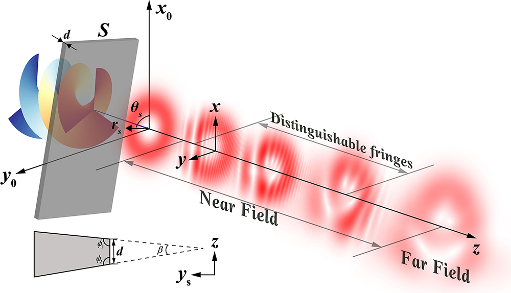
Assuming a paraxial monochromatic Gaussian-background vortex beam propagating along axis $z$ is normally incident at a screen plate (depicted as Fig. 1), the complex amplitude of the beam at $z = 0$ can be described by^[31] $u_{0} (x_{0}, y_{0}, 0) \equiv u_{0} (x_{0}, y_{0}) = A {(x_{0} + i σ y_{0})}^{| l |} \exp (- \frac{x_{0}^{2} + y_{0}^{2}}{w_{0}^{2}}),$ (1)where $w_{0}$ is the waist width of the Gaussian beam, $σ = sgn (l)$ , $l$ is the TC, and $A$ is a constant.

$Scheme of TC measurement of a vortex beam (l = 3 exampled) with a screen plate S located at the x0−y0 plane (z = 0). The cross section of the plate is shown at the bottom left. The diffraction patterns aligned along the z axis illustrate the evolution of the OV edge diffraction.$

Figure 1.Scheme of TC measurement of a vortex beam (l = 3 exampled) with a screen plate S located at the x₀−y₀ plane (z = 0). The cross section of the plate is shown at the bottom left. The diffraction patterns aligned along the z axis illustrate the evolution of the OV edge diffraction.

Considering that the screen plate located at the x₀−y₀ plane is rectilinear hard-edged, and the size of the plate is much larger than the beam waist (shown as Fig. 1), then the transmittance function of the plate can read $T (x_{0}, y_{0}) = {\begin{cases} 1, & x_{0} \cos θ_{s} + y_{0} \sin θ_{s} < r_{s} \\ α \exp (i Φ), & else \end{cases},$ (2)where $θ_{s}$ is the azimuthal angle of the plate edge (counted in the anti-clockwise direction), and $r_{s} (\geq 0)$ is the distance from the origin to the plate edge. $Φ = n k d$ is the additional phase associated with the thickness of the plate, where $α, n, d$ are the transparency, refractive index, and thickness of the plate, respectively. Equation (2) can degenerate into an ordinary opaque plate when $α = 0$ or a transparent homogeneous phase step with $α = 1$ . Generally, the front and rear surfaces are not technically parallel. Therefore, the phase step can be viewed as a prism with top angles of $ϕ_{1}$ and $ϕ_{2}$ (shown in Fig. 1), and then the thickness $d$ should be replaced by $d (x_{s}) = d_{0} - \frac{\sin (ϕ_{1} + ϕ_{2})}{\sin (ϕ_{1}) \sin (ϕ_{2})} (x_{s} - r_{s}),$ (3)where $d_{0}$ is the thickness of the substrate, and $(x_{s}, y_{s})$ is the coordinate frame rotated with $θ_{s}$ from $(x_{0}, y_{0})$ giving relations $x_{s} = x_{0} \cos θ_{s} - y_{0} \sin θ_{s}, y_{s} = x_{0} \sin θ_{s} + y_{0} \cos θ_{s} .$ (4)

Particularly, when the cross section of S is an isosceles trapezoid, i.e., $ϕ_{1} = ϕ_{2}$ , the angle formed by the intersection of the extended lines on both sides of the trapezoid gives $β = ϕ_{1} + ϕ_{2} - π$ . Then, Eq. (3) evolves to $d (x_{s}) = d_{0} + 2 \tan (β / 2) (x_{s} - r_{s}) .$ (5)

After the edge diffraction, the light field gives the complex amplitude at the distance of $z$ determined by the Fresnel diffraction integral in the Kirchhoff–Fresnel approximation $u (x, y, z) = \frac{e^{- i k z}}{i λ z} \int_{- \infty}^{\infty} d y_{0} \int_{- \infty}^{\infty} u_{0} (x_{0}, y_{0}) T (x_{0}, y_{0}) d x_{0} \times \exp {\frac{i k}{2 z} [{(x - x_{0})}^{2} + {(y - y_{0})}^{2}]} .$ (6)

Equation (6) can be changed to the form of Fourier transformation $u (x, y, z) = \frac{e^{- i k z}}{i λ z} \exp [\frac{i k}{2 z} (x^{2} + y^{2})] \times F {u_{0} (x_{s}, y_{s}) T (x_{s}, y_{s}) e^{\frac{i k}{2 z} (x_{s}^{2} + y_{s}^{2})}} = E (x, y, z) \cdot [u_{1} (x, y, z) + α u_{2} (x, y, z)],$ (7)where $E (x, y, z) = A e^{i l θ_{s}} \frac{e^{- i k z}}{i λ z} \exp [i k (\frac{x^{2} + y^{2}}{2 z})],$ (8) $u_{1} (x, y, z) = \int_{- \infty}^{\infty} d y_{s} \int_{- \infty}^{r_{s}} d x_{s} {(x_{s} + i σ y_{s})}^{| l |} \times \exp [(\frac{i k}{2 z} - \frac{1}{w_{0}^{2}}) (x_{s}^{2} + y_{s}^{2})] \times \exp [- \frac{i k}{z} (x x_{s} + y y_{s})],$ (9) $u_{2} (x, y, z) = \int_{- \infty}^{\infty} d y_{s} \int_{r_{s}}^{\infty} d x_{s} {(x_{s} + i σ y_{s})}^{| l |} e^{i n k d (x_{s})} \times \exp [(\frac{i k}{2 z} - \frac{1}{w_{0}^{2}}) (x_{s}^{2} + y_{s}^{2})] \times \exp [- \frac{i k}{z} (x x_{s} + y y_{s})],$ (10)and $F {\cdot}$ denotes the spatial Fourier transform. The intensity distribution can be calculated with $I = 〈 u \cdot u^{*} 〉$ . The last line of Eq. (7) shows that the diffraction can be considered as the superimposition of $u_{1}$ and $u_{2}$ , and $α$ represents the weight of $u_{2}$ . In this consideration, $u_{1}$ [see Eq. (9)] leads to the edge diffraction of an opaque screen, and $u_{2}$ offers the blocked OV diffraction of a rectilinear phase step with the addition phase of $n k d (x_{s})$ . Note that the integrals of Eqs. (9) and (10) can be deduced into analytical expressions that are pretty complicated^[32], and numerical methods such as the fast Fourier transform (FFT) algorithm used in this paper are more convenient to simulate and analyze the evolution of the partially blocked OV beams.

3. Simulation Results of the Edge Diffraction

3.1. Opaque screen

The edge diffraction by an opaque screen ( $α = 0$ ) has verified that the creation, motion, and annihilation of phase singularities in the diffraction field may appear by varying the edge deviation and propagation distance^[25,28,30].

Note that the radius of the OV beam at the maximum of intensity is associated with its TC ( $l$ ) and waist radius ( $w_{0}$ at $z = 0$ ) of the fundamental mode, given by $r_{\max} = \sqrt{| l | / 2} w_{0} .$ (11)

Here, we define the normalized deviation of the plate edge as $\bar{r} = r_{s} / r_{\max}$ and the normalized diffraction distance as $\bar{z} = z / z_{R}$ , where $z_{R} = π w_{0}^{2} / λ$ is the Rayleigh distance of the Gaussian beam.

Figure 2 calculated via Eq. (8) shows the simulated intensity distributions of the edge diffraction of a blocked OV beam with an opaque screen. The wavelength used in the simulation is 1064 nm, and the waist radius is 1 mm, giving $z_{R} = 5.91 m$ . Diffraction patterns of varied TCs are shown in Fig. 2(a). It is verified that OV beams embedded with phase singularities exhibit redundant fringes in contrast with the straight fringes of the conventional Gaussian beam. For $l > 0$ , the redundant fringes appear at the top when the screen blocks partial light on the right, i.e., the ‘fork’ orients to the upper and vice versa, where the number of the redundant fringes is equivalent to $| l |$ . Note that the deviation of the edge may result in different diffraction patterns. It is recommended from simulation results [shown in Fig. 2(b)] that the rightmost fringe should be preserved in order to determine which fringes are redundant. On the other hand, as the fifth column of Fig. 2(b) shows, the diffraction fringes vanish when the screen edge locates more than $2 r_{\max}$ ( $\bar{r} \geq 2$ ) away from the center, which shows the weak influence of the edge. Therefore, to obtain distinct fringes, the edge of the screen plate can deviate about $0.5 r_{\max} - 1.5 r_{\max}$ from the center of the OV beam.

$Simulated intensity profiles of OV beams edge-diffracted by an opaque screen for (a) l = −2 to 2 in steps of 1, (b) r¯=0–2 in steps of 0.5, (c) θs = 0°–180° in steps of 45°, and (d) z¯=0.05, 0.1, 0.2, 0.4, 1, respectively. The general case is l = 3, r¯=1, θs = 0°, and z¯=0.1. Auxiliary red dashed lines indicate the dark fringes. Hatched area shows the position of the plate, and the yellow arrow points in the direction of the fork-shaped fringe. The intensity distribution is normalized.$

Figure 2.Simulated intensity profiles of OV beams edge-diffracted by an opaque screen for (a) l = −2 to 2 in steps of 1, (b) r¯ $= 0 - 2$ in steps of 0.5, (c) θ_s = 0°–180° in steps of 45°, and (d) z¯ $= 0.05$ , 0.1, 0.2, 0.4, 1, respectively. The general case is l = 3, r¯ $= 1$ , θ_s = 0°, and z¯ $= 0.1$ . Auxiliary red dashed lines indicate the dark fringes. Hatched area shows the position of the plate, and the yellow arrow points in the direction of the fork-shaped fringe. The intensity distribution is normalized.

It is shown in Fig. 2(c) that the pattern rotates as the edge rotates due to the rotational symmetry of the OV beam. Thus, the orientation of the fork-shaped pattern should be defined relative to the screen edge. The evolution of the diffraction pattern along the $z$ axis with varied diffraction distances $z$ is depicted in Fig. 2(d) with the normalized values of $\bar{z} = 0.05$ , 0.1, 0.2, 0.4, and 1 for column 1–5, respectively. It turns out that the number of the fringes decreases as the edge-diffracted beam propagates further, and the fringes are finally deformed into a symmetric structure, in which the symmetry axis is parallel to the edge of the screen. This phenomenon is consistent with the theoretical and experimental results in early works^[25–27]. The overall requirement to discernibly and effectively measure the TC and the handedness of the incident OV beam is that the diffraction distance and the edge deviation are suggested to be controlled at $z = (0.05 - 0.4) z_{R}$ and $r = (0.5 - 2) r_{\max}$ , respectively.

3.2. Translucent plate

As the screen plate becomes transparent (Fig. 3), the blocked part goes through an additional phase $Φ = n k d$ [see also Eq. (2)]. Figure 3(b) shows the varied normalized thickness $\bar{d} = 8 \cdot \mod (n d, λ) / λ = 0 - 4$ , giving the additional phase $Φ = 2 π m + π \bar{d} / 4 = 2 π m + (0 - 1) π$ , where $m$ is an integer. A phase step is formed between the perturbed and ‘survived’ segments of the vortex beam and exhibits strong perturbation when the phase step value approaches $π$ or $\bar{d} = 4$ in Fig. 3(b)^[32]. In this case, the two segments of the vortex beam interfere to the maximum extent. At the same time, the fork-shaped fringes can be more discernible. Therefore, the angle $β$ between two surfaces of the plate can be used to adjust the position of the perturbed segment (see Fig. 1). As Fig. 3(c) shows, the fringes are further distinct when the perturbed segment is at the center of the OV beam, for instance, $β = - 3 °$ at $\bar{z} = 0.1$ in Fig. 3(c).

$Simulated intensity profiles at l = 3, r¯=1, z¯=0.1 after edge diffraction by a translucent plate with (a) the transparency α = 0–1 in steps of 0.25, (b) the normalized thickness d¯=0–4 in steps of 1, and (c) the angle between two surfaces of the plate β = −6° to 6° in steps of 3°. The general case is α = 1, d¯=4, and β = 0°.$

Figure 3.Simulated intensity profiles at l = 3, r¯ $= 1$ , z¯ $= 0.1$ after edge diffraction by a translucent plate with (a) the transparency α = 0–1 in steps of 0.25, (b) the normalized thickness d^¯ $= 0 - 4$ in steps of 1, and (c) the angle between two surfaces of the plate β = −6° to 6° in steps of 3°. The general case is α = 1, d^¯ $= 4$ , and β = 0°.

4. Experiment Results and Discussions

The edge-diffraction-based TC measurement is also experimentally demonstrated, and the setup is shown in Fig. 4(a). A neodymium-doped yttrium aluminum garnet (Nd:YAG) laser is used to produce the fundamental Gaussian mode at $λ = 1064 nm$ with the waist radius $w_{0} = 0.685 mm$ and then expanded into 1.5 mm by an expander, giving the Rayleigh distance $z_{R} = 6.643 m$ . The incident beam illuminates a pure phase SLM loaded with fork-shaped blazed gratings [shown in Fig. 4(b)], generating the desired OV beam at the first diffraction order, and the other orders are filtered with an iris diaphragm.

Figure 4.(a) Experimental setup for generating the OV beam using SLM1 loaded with (b) fork-shaped blazed gratings and measuring the TC using SLM2 loaded with (c) a phase step. λ/2, half-wave plate; SLM, spatial light modulator; S, an opaque screen in Fig. 1 in the case of α = 0; CCD, charge coupled device.

As shown in Fig. 4(a), in the case of $α = 0$ , an opaque screen S is employed to realize the hard edge diffraction. For $α = 1$ , as a consequence of the additional phase $Φ = 2 π n d / λ$ varying with a period of $2 π$ , it is challenging to control the plate thickness in the wavelength scale (the effective optical thickness $d = \bar{d} λ / 4 n$ , $\bar{d} = 0 - 4$ ). Therefore, in this experiment, S is substituted by another SLM (SLM2) loaded with a phase step [shown in Fig. 4(c)] to mimic the transparent plate. On the other hand, the phase pattern in SLM2 is supposed to be a whiteboard when switching to the opaque screen diffraction. Finally, a CCD camera set at the distance of $z$ from S or SLM2 is used to capture the diffraction profiles.

Figure 5 shows the experimental results of the truncated OV beam of $l = 3$ with varied edge deviations of an opaque or a transparent plate. Note that there are several ‘ripples’ in the generated beam, and the ring width is narrower than that desired in Fig. 2. It may result from the properties of the Kummer beam^[33], which is usually generated by fork-shaped gratings and can be degraded into a sum of standard LG beams with different TCs and weights. Regardless, the experimental fringes in Fig. 5(b), to a certain extent, show good agreement with the simulation ones in Fig. 2(b). Figures 5(a)–5(c) show that the fringes can remain discernible at $\bar{r} = 0.5 - 1.5$ and $\bar{z} = 0.05 - 0.2$ , i.e., $r_{s} = 0.48 - 1.44 mm$ and $z = 33.22 - 132.86 cm$ in our experiment, which is a wide range in three-dimensional space.

$Experimental intensity profiles of the OV beam (l = 3) at z¯ of (a) 0.05, (b), (d) 0.1, and (c) 0.2 after edge diffraction by (a)–(c) an opaque or (d) a transparent plate (d¯=4) at r¯=0–1.5 in steps of 0.5 for column 1–4, respectively.$

Figure 5.Experimental intensity profiles of the OV beam (l = 3) at z¯ of (a) 0.05, (b), (d) 0.1, and (c) 0.2 after edge diffraction by (a)–(c) an opaque or (d) a transparent plate (d^¯ $= 4$ ) at r¯ $= 0 - 1.5$ in steps of 0.5 for column 1–4, respectively.

In addition, the edge-diffraction patterns of the transparent plate at $\bar{z} = 0.1$ with fixed $\bar{d} = 4$ and varied $\bar{r}$ are shown in Fig. 5(d). By contrast with those of the opaque screen in Fig. 5(b), it can be seen that the actual interference of the two segments of the vortex beam mentioned in Section 3.2 is not obvious enough to improve the fringe clarity. It may still result from the narrow ring width of the Kummer beam so that the light from the blocked segment is not enough to interfere with the other.

The experimental results for the measurement of higher TCs of OV beams with $l = \pm 40$ (compared to $| l | \leq 3$ illustrated above) by an opaque screen are shown in Fig. 6. Since the central dark area of OV light becomes more expansive with the increase of TC, coupled with the ratchet-shaped initial light-field background [shown as Fig. 6(a)] caused by insufficient SLM resolution, fringes of the edge diffraction become more inconspicuous. Therefore, for measurements of high TCs, the background profile of the generated OV beam is removed from the fringes of the edge-diffraction pattern to enhance the fringe contrast. Figure 6(c) shows the corresponding enhanced fringes where one can explicitly count the number of bright stripes at the upper and lower cambered cross section of the intensity, and specific values are shown in Fig. 6(d). As the plate is set to the right of the OV beam, the TC value can be determined by subtracting the number of lower fringes from the number of upper fringes. In this case, the subtracted number’s sign coincides with the chirality of the vortex beam to be measured.

$Experimental intensity profiles for (a) unperturbed and (b) opaque screen (r¯=1, z¯=0.1) edge-diffracted vortex beams with topological charge −40 and +40 for columns 1 and 2, respectively. Corresponding enhanced patterns are shown in (c), where the inset with the yellow box shows the partially scaled image, and the cambered red and blue cross sections of the intensity indicate (d) the number of upside and downside fringes, respectively.$

Figure 6.Experimental intensity profiles for (a) unperturbed and (b) opaque screen (r¯ $= 1$ , z¯ $= 0.1$ ) edge-diffracted vortex beams with topological charge −40 and +40 for columns 1 and 2, respectively. Corresponding enhanced patterns are shown in (c), where the inset with the yellow box shows the partially scaled image, and the cambered red and blue cross sections of the intensity indicate (d) the number of upside and downside fringes, respectively.

This method can remain steady for much higher TC measurements but is limited by the resolution and field of view of the CCD due to the increasing ring size and fringe density at the end away from the plate edge. In this case, one can extend the diffraction distance or reduce the edge deviation from the center to increase the stripe spacing.

5. Conclusion

In conclusion, it is demonstrated theoretically and experimentally that the edge of a plate can be used to measure the TC of OV beams at a proper diffraction distance in the near-field. The number of redundant fringes in the diffraction fork-shaped pattern is equal to the TC value, and the orientation of the fork relative to the plate edge indicates the handedness of the OV beam. Simulated results of the opaque screen indicate that the diffraction fringe contrast increases when the screen edge moves closer to the center of the OV beam, and the fringe density decreases as the diffraction distance increases, forming a three-dimensional space to control the diffraction fringes. It turns out that the edge diffraction of translucent plates can also be used to form fork fringes based on the self-interference of the OV beam with a rectilinear phase step. The transparency of the plate affects the degree of interference, and the angle between two surfaces of the plate determines the interference angle. However, experimental results do not show obvious self-interference from the simulation due to the intensity differences between the generated Kummer beam and the standard LG beam. Since the generated OV beam with high TCs is accompanied by the intrinsic large central dark area and low purity limited by the SLM resolution, the additional computational diffraction fringe enhancement by removing the background profile of the undiffracted beam from the diffraction pattern is recommended and applied in our analysis for $l = \pm 40$ .

This TC measurement method for OV beams takes good advantage of using only one simple and easily available screen whether it is opaque or not. As the edge-diffraction pattern is relevant to the phase of the incident light field, the method could be used to diagnose the phase structure and energy flow for other OV beams, such as composed vortices (a method to measure fractional TC has been proposed in Ref. [34]) and vector vortices^[35,36].

References

[1] L. Allen, M. W. Beijersbergen, R. J. Spreeuw, J. P. Woerdman. Orbital angular momentum of light and the transformation of Laguerre–Gaussian laser modes. Phys. Rev. A, 45, 8185(1992).

[2] D. G. Grier. A revolution in optical manipulation. Nature, 424, 810(2003).

[3] J. Ng, Z. Lin, C. T. Chan. Theory of optical trapping by an optical vortex beam. Phys. Rev. Lett., 104, 103601(2010).

[4] G. Gibson, J. Courtial, M. J. Padgett, M. Vasnetsov, V. Pas’ko, S. M. Barnett, S. Franke-Arnold. Free-space information transfer using light beams carrying orbital angular momentum. Opt. Express, 12, 5448(2004).

[5] A. Nicolas, L. Veissier, L. Giner, E. Giacobino, D. Maxein, J. Laurat. A quantum memory for orbital angular momentum photonic qubits. Nat. Photonics, 8, 234(2014).

[6] G. C. Berkhout, M. W. Beijersbergen. Method for probing the orbital angular momentum of optical vortices in electromagnetic waves from astronomical objects. Phys. Rev. Lett., 101, 100801(2008).

[7] J. Leach, M. J. Padgett, S. M. Barnett, S. Franke-Arnold, J. Courtial. Measuring the orbital angular momentum of a single photon. Phys. Rev. Lett., 88, 257901(2002).

[8] H. I. Sztul, R. R. Alfano. Double-slit interference with Laguerre–Gaussian beams. Opt. Lett., 31, 999(2006).

[9] M. V. Vasnetsov, V. V. Slyusar, M. S. Soskin. Mode separator for a beam with an off-axis optical vortex. Quantum Electron., 31, 464(2001).

[10] P. Kumar, N. K. Nishchal. Modified Mach–Zehnder interferometer for determining the high-order topological of Laguerre–Gaussian vortex beams. J. Opt. Soc. Am. A, 36, 1447(2019).

[11] P. Kumar, N. K. Nishchal. Self-referenced interference of laterally displaced vortex beams for topological charge determination. Opt. Commun., 459, 125000(2020).

[12] A. Lubk, G. Guzzinati, F. Borrnert, J. Verbeeck. Transport of intensity phase retrieval of arbitrary wave fields including vortices. Phys. Rev. Lett., 111, 173902(2013).

[13] J. M. Hickmann, E. J. Fonseca, W. C. Soares, S. Chavez-Cerda. Unveiling a truncated optical lattice associated with a triangular aperture using light’s orbital angular momentum. Phys. Rev. Lett., 105, 053904(2010).

[14] D. P. Ghai, P. Senthilkumaran, R. S. Sirohi. Single-slit diffraction of an optical beam with phase singularity. Opt. Lasers Eng., 47, 123(2009).

[15] H. Tao, Y. Liu, Z. Chen, J. Pu. Measuring the topological charge of vortex beams by using an annular ellipse aperture. Appl. Phys. B, 106, 927(2012).

[16] S. N. Alperin, R. D. Niederriter, J. T. Gopinath, M. E. Siemens. Quantitative measurement of the orbital angular momentum of light with a single, stationary lens. Opt. Lett., 41, 5019(2016).

[17] P. Vaity, J. Banerji, R. P. Singh. Measuring the topological charge of an optical vortex by using a tilted convex lens. Phys. Lett. A, 377, 1154(2013).

[18] K. Dai, C. Gao, L. Zhong, Q. Na, Q. Wang. Measuring OAM states of light beams with gradually-changing-period gratings. Opt. Lett., 40, 562(2015).

[19] Z. Liu, S. Gao, W. Xiao, J. Yang, X. Huang, Y. Feng, L. I. Jianping, L. I. U. Weiping, L. I. Zhaohui. Measuring high-order optical orbital angular momentum with a hyperbolic gradually changing period pure-phase grating. Opt. Lett., 43, 3076(2018).

[20] S. Fu, T. Wang, Y. Gao, C. Gao. Diagnostics of the topological charge of optical vortex by a phase-diffractive element. Chin. Opt. Lett., 14, 080501(2016).

[21] S. Rasouli, S. Fathollazade, P. Amiri. Simple, efficient and reliable characterization of Laguerre–Gaussian beams with non-zero radial indices in diffraction from an amplitude parabolic-line linear grating. Opt. Express, 29, 29661(2021).

[22] I. V. Basistiy, V. K. Lyubov, I. G. Marienko, S. S. Marat, V. V. Mikhail. Experimental observation of rotation and diffraction of a singular light beam. Proc. SPIE, 3487, 34(1998).

[23] I. G. Marienko, M. S. Soskin, M. V. Vasnetsov. Diffraction of optical vortices. Fourth International Conference on Correlation Optics, 27(1999).

[24] J. Masajda. Gaussian beams with optical vortex of charge 2- and 3-diffraction by a half-plane and slit. Opt. Appl., 30, 247(2000).

[25] A. Y. Bekshaev, K. A. Mohammed. Spatial profile and singularities of the edge-diffracted beam with a multicharged optical vortex. Opt. Commun., 341, 284(2015).

[26] J. Arlt. Handedness and azimuthal energy flow of optical vortex beams. J. Mod. Opt., 50, 1573(2003).

[27] A. Y. Bekshaev, K. A. Mohammed, I. A. Kurka. Transverse energy circulation and the edge diffraction of an optical vortex beam. Appl. Opt., 53, B27(2014).

[28] H. X. Cui, X. L. Wang, B. Gu, Y. N. Li, J. Chen, H. T. Wang. Angular diffraction of an optical vortex induced by the Gouy phase. J. Opt., 14, 055707(2012).

[29] R. Chen, X. Zhang, Y. Zhou, H. Ming, A. Wang, Q. Zhan. Detecting the topological charge of optical vortex beams using a sectorial screen. Appl. Opt., 56, 4868(2017).

[30] P. Liu, B. Lü. Propagation of Gaussian background vortex beams diffracted at a half-plane screen. Opt. Laser Technol., 40, 227(2008).

[31] F. Flossmann, U. T. Schwarz, M. Maier. Propagation dynamics of optical vortices in Laguerre–Gaussian beams. Opt. Commun., 250, 218(2005).

[32] A. Bekshaev, A. Khoroshun, L. Mikhaylovskaya. Transformation of the singular skeleton in optical-vortex beams diffracted by a rectilinear phase step. J. Opt., 21, 084003(2019).

[33] A. Y. Bekshaev, A. I. Karamoch. Spatial characteristics of vortex light beams produced by diffraction gratings with embedded phase singularity. Opt. Commun., 281, 1366(2008).

[34] S. M. A. Hosseini-Saber, E. A. Akhlaghi, A. Saber. Diffractometry-based vortex beams fractional topological charge measurement. Opt. Lett., 45, 3478(2020).

[35] Z. Man, Z. Xi, X. Yuan, R. Burge, H. P. Urbach. Dual coaxial longitudinal polarization vortex structures. Phys. Rev. Lett., 124, 103901(2020).

[36] A. Holleczek, A. Aiello, C. Gabriel, C. Marquardt, G. Leuchs. Classical and quantum properties of cylindrically polarized states of light. Opt. Express, 19, 9714(2011).