Ghost imaging (GI) provides a way to obtain images with a single-pixel detector, employing second-order correlation between the illumination field and the signal from the object. Since the first realization with entangled photons^[1–3], researchers made great developments in different aspects^[4–14], showing its ability for lensless imaging^[15] and robustness against noise^[16,17], and exploring possible applications in different fields^[18–24]. With the illumination patterns actively controlled and computed, the detector in the reference arm can be omitted, which further simplified the system into a real single-pixel imaging system. This is called computational GI^[25–28]. Due to the feature of correlation, a large number of measurements are required to achieve high-quality images, which limits the performance of GI. Many methods^[29–35] have been proposed towards this issue. Based on the sparsity of the interested scene, compressive GI (CSGI)^[30,31] has been proved to be an effective method to decrease the number of required samplings, with the cost of heavy computing consumption. Then, adaptive GI methods based on compressed sensing and wavelet trees^[31–33] were reported to slow down the growth of computing consumption over the size of the image. However, complicated data processing algorithms are still required, which also costs additional time after data sampling. Therefore, methods that can decrease both the number of required measurements and computation consumption are crucial for real-time imaging.

In conventional GI, every pixel within the illuminated scene is treated evenly, without considering how much information is required to properly describe it. Towards this, researchers performed GI in an adaptive way, by adjusting illumination patterns according to previous results^[36–39]. As is observed, the edge areas of the objects contain the most details, and thus more information is required to clearly reconstruct the image of those areas. At the same time, the temporal–spatial distribution of speckles determines the information we can achieve from the target. If we divide the imaging process into different stages and gradually find out it and concentrate on the edge area, it is possible to improve effective information obtained via each measurement. Based on this idea, we propose a method named edge lit feedback GI (ELFGI) to adaptively adjust the field of view and the average size of speckles according to the previous images; thus, the illumination area providing higher spatial resolution is gradually concentrated onto the edge area. The image of the scene is gradually becoming distinct, while the number of required samplings is greatly reduced compared to conventional GI. Data processing is performed along with data acquisition, using a linear algorithm.

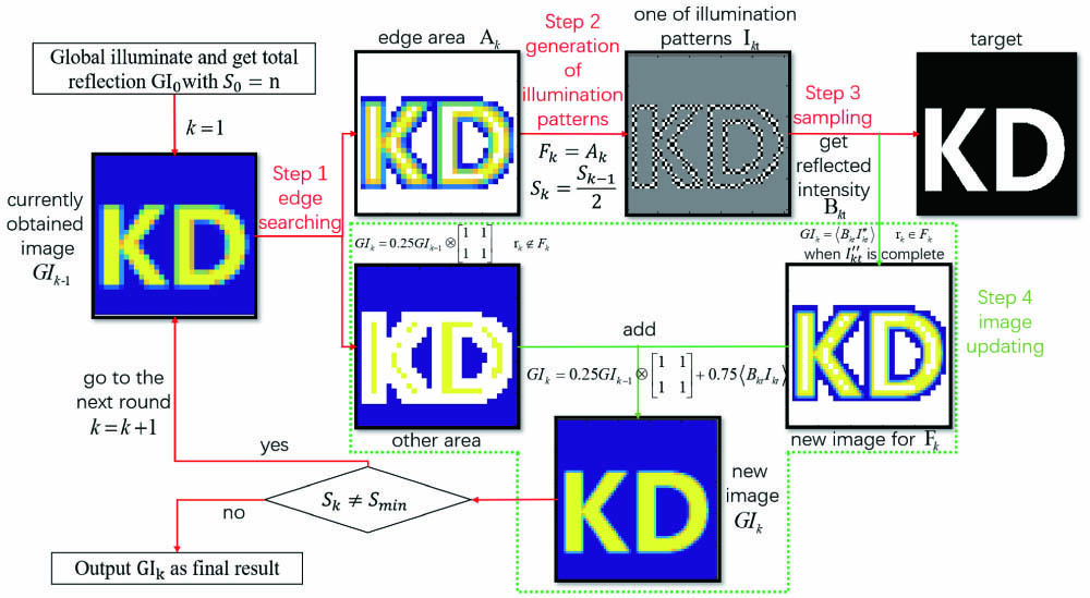
In a typical GI system, a sequence of patterns are illuminated onto the object, with the counterpart echoes from the object detected with the bucket detector; then the correlation between these patterns and the detection results provides the image. In our scheme, the sequence of patterns is adaptively arranged. According to different settings of the illumination patterns, the whole imaging process is divided into many rounds. For each round, four steps are performed, namely, edge searching, pattern generation, sampling, and image updating. Firstly, we consider binary sparse objects for convenience. The scene is described as O, with the size of n×n. We use Fk to denote the field of view, and Sk to denote the size of speckles in the kth round. In every round, an image GIk(r→k) of size nSk×nSk is reconstructed. Here, r→k is the coordinate in the image, and the resolution is Sk. Every value in GIk actually shows the total reflection within the block with the size of Sk. GIk is then used as the input of the next round. A flow diagram is shown in Fig. 1. To start, we light up the whole scene and measure the reflected intensity of the target as GI0, the resolution of which is S0=n. Then, the imaging process moves forward to the rounds containing the following four steps.

Step 1: edge searching. For binary targets, the grayscale values within the object (background) areas are close to the maximum (minimum), with noise involved. If these areas are picked out, the rest of the area is the edge area. Considering white Gaussian noise in bucket detection with the standard deviation σ, the standard deviation of the error in every pixel of the currently obtained image GIk−1 is σNk, with Nk being the total number of performed measurements. Considering the errors, we can pick out the edge areas Ak, which are defined as the set of r→k−1, which satisfies min(GIk−1)+ϵ<GIk−1(r→k−1)<max(GIk−1)−ϵ.(1)Here, ϵ=TNk actually defines the tolerance of errors, and T is set as a constant, since σ can be taken as unchanged during each experiment. In practice, σ can be estimated from the fluctuation of the bucket detection under the same illumination, and T is set as 6σ. Higher T promises higher confidence that the selected part belongs to the edge area.

Step 2: generation of illumination patterns. Since the image obtained in each round is used as the input of the next round, the quality of the image will be important for edge searching. GI with Hadamard patterns^[40,41] provides an image of high accuracy with complete samplings. Therefore, we use the Hadamard matrix as the basic pattern, with each row of the matrix being one frame of the illumination pattern, and perform complete samplings for each round to achieve an image of as high quality as possible. Since the size of speckles is large when the field of view is large, and the field of view is concentrated to the edge area when the size of speckles becomes small, a large number of frames are not required, as will be shown later. Each element in GIk−1 corresponds to the reflection of a block with the size of Sk−1. Ak is also constituted with such blocks. To obtain more details about the edge area, the resolution should be improved, which means the speckles in the new masks should be smaller than those of the previous rounds. Each block in Ak with the size of Sk−1 is divided evenly into four squares, with every square being a new block in this round. The size of the blocks is Sk=Sk−1/2 with the coordinates updated into r→k. When used to generate the masks, each element of the Hadamard matrix describes the intensity of the counterpart block in the mask. As defined, the number of elements in each mask is 2m(m∈N+). To match the illumination area Fk with the determined edge area Ak, we set mk=max(⌈log2nk′⌉,2), where nk′ is the number of blocks contained in Ak. That is, we set the illumination matrix to be the smallest Hadamard matrix that can cover the edge area, and every block in Ak is a speckle in Fk. As the number of speckles in Fk is nk=2mk, a Hadamard matrix of 2mk×2mk can be used to generate the masks, according to the recursion relationship^[41]: Hmk=(11111−11−111−1−11−1−11)⊗Hmk−2=(hk(1)hk(2)hk(3)hk(4)),(2)where Hmk−2 is the Hadamard matrix of 2mk−2×2mk−2, and hk(j)(j=1,⋯,4) contains 0.25nk rows of Hmk, respectively. ⊗ here represents the operation of the Kronecker product. In traditional Hadamard GI, each row of Hmk−2 is reshaped into an illumination mask Ikt″. Since the measurement matrix hk(1) is equivalent to Hmk−2, which represents those patterns of the last round with GIk−1 being the imaging result, only the parts containing hk(2), hk(3), and hk(4) are necessary in the current round, with each row reshaped into an illumination mask Ikt.

Step 3: sampling. Ikt determined in the previous step are the expected masks, which contain negative values. In practice, the values of −1 in Ikt are changed into zero, as Ikt′=(Ikt+1)/2,r→k∈Fk.(3)Here, Ikt′ is the actually performed illumination. Then, the reflected intensity is measured and written as Bkt′=∑r→kIkt′(r→k)O,r→k∈Fk.(4)Therefore, Bkt corresponding to the expected illumination Ikt can be obtained as Bkt=∑r→k(2Ikt′−1)O=2Bkt′−∑r→kGIk−1,r→k∈Fk,(5)where we use GIk−1 to replace O within Fk, as GIk−1 is actually the measured reflection of the target from previous rounds, while O is the real reflection.

Step 4: image updating. The new image GIk is constituted by two parts, the area in and out of Fk. For the area in Fk, GIk=〈BktIkt″〉 as Ikt″ corresponds to the whole Hmk. GIk−1, with the size expanded, is used to take the role of hk(1), which occupies one quarter of Hmk in our method. Thus, GIk can be reconstructed with GIk=0.25GIk−1⊗[1111]+0.75〈BktIkt〉.(6)

For the area out of Fk, the value on each pixel of GIk equals one quarter of GIk−1 at the same position, due to the size changing of speckles. Since Ikt(r→k∉Fk)=0, Eq. (6) also works for the region out of Fk, from which the image GIk is updated for the whole scene.

After Step 4, if Sk has reached the limit of the imaging system, the whole imaging process is finished, and GIk is taken as the final result; otherwise, move to Step 1 for the next round.

To implement our method, we build a very simple setup, as shown in Fig. 2. A commercial projector (Panasonic PT-X301) is employed as the source, which outputs different masks with 256×256 pixels, controlled by a laptop. The size of each pixel is 0.24 mm × 0.24 mm on the object plane, which is 45 cm away from the output lens of the projector. The reflected light by the target is collected with a lens and detected by a CCD camera. For each frame, the values on all pixels of the camera are summed up and quantified to 0–255 as the bucket detection. Data acquisition and data processing are performed simultaneously. After each round, the edge area is picked out with the laptop, and then new illumination patterns for the next round are generated, which will be imprinted on the object plane to update the image.

The objects used in our experiments are made by cutting a piece of paper into Chinese characters, as shown in Figs. 3(a1) and 3(c1). The images retrieved in the 4th–7th rounds with ELFGI are shown in Figs. 3(b1)–3(b4) and 3(d1)–3(d4). The reconstructed images become distinguishable after four rounds, clearer and clearer. The edge area, which is also the field of view, is getting smaller and smaller. The number of pixels illuminated in the 4th–7th rounds is 16,384, 8192, 8192, and 4096, respectively. The resolution is increased as average sizes of the speckles at the 4th–7th round are 16, 8, 4, and 2 pixels, with the corresponding number of speckles within the illumination area being 64, 128, 512, and 1024, respectively. The total number of performed illumination patterns is 70, 166, 550, and 1318, respectively. The images shown in Figs. 3(a2)–3(a4) and 3(c2)–3(c4) are the results of conventional GI with 2000 frames using random speckles, and the average sizes of the speckles are 16, 4, and 2 pixels, respectively. It can be seen that the images retrieved with our method appear to be with higher quality than that of conventional GI. To quantitatively compare those results, the mean square error (MSE) is considered, defined as MSE=1n2∑r→k[GI(r→k)−O]2. The reference O is obtained with traditional imaging. The results via ELFGI become clear fast when MSE drops sharply. The result is very close to the target after seven rounds, with the MSE being 0.0075. With the same number of measurements, the MSEs of conventional GI are 0.24, 0.11, and 0.041 when the average sizes of speckles are 16, 4, and 1 pixel(s). From these results, it is verified that our method helps get an image of higher quality with fewer samplings with a simple retrieving algorithm. Thus, the process of GI can be accelerated with our method.

Actually, our method also provides a way to remove the trade-off between high resolution and high signal-to-noise ratio (SNR)^[42], both of which require a large number of samplings. To demonstrate this, we do simulations for the chart with objects of different sizes, as shown in Fig. 4(a1). Results from different methods are shown in Figs. 4(a2)–4(a4). It takes 65,536 samplings for GI with Hadamard patterns. For conventional GI with random speckles, the narrowest stripes are still barely visible with 47,104 samplings. With our method, fewer samplings (4480) are required to achieve the expected resolution. Therefore, the requirement on a high number of samplings for high resolution is greatly reduced.

Our method can also work for grayscale objects, with the algorithm of edge searching adapted. We simulate imaging an object of three-level grayscale values, as shown in Fig. 4(b1). To find out the edge area, the Canny operator algorithm is used. The imaging results are shown in Figs. 4(b2)–4(b4). With eight rounds and 6016 samplings in total, an image of 256×256 is perfectly retrieved. That is, our method has the capacity to reconstruct grayscale images with the number of required samplings reduced.

The performance of our method under noise is also explored with simulations, with the results shown in Fig. 5. The SNR of the bucket detection, defined as the ratio between the average value of the bucket detection and the standard deviation σ of noise, is used to measure the influence of noise. The amount of required samplings is proportional to σ2 for traditional GI to get the image of certain quality. As for ELFGI, we change T according to the noise and repeat measurements in the first five rounds to increase reliability of the measurement. Although a decline in the quality is unavoidable, the image is distinguishable using ELFGI or CSGI. From the results, with a comparable number of measurements, the imaging quality of CSGI is a little better than of ELFGI. However, the time cost for extra calculation in CSGI (90 s for 4500 samplings using a laptop with CPU of E5-2667 at 3.30 GHz) is hundreds of times longer than that of ELFGI (0.39 s). The algorithm of CSGI used here is a gradient projection for sparse reconstruction.

Experimentally, we are using a commercial projector, which makes the experiments easier to perform. Such projectors are usually not fast enough for real-time imaging. By modulating a laser with a digital micro-mirror device (DMD) or a spatial light modulator (SLM), the refresh rate of the source can be improved. Then, the sampling rate and the minimum resolution of GI can be improved. The time consumption of the calculation can also be reduced by hardware design. Therefore, our method makes GI closer to practical applications, since fewer samplings are required. Although we employed Hadamard illumination patterns in our discussion and experiments, the design and selection of illumination patterns are not confined. The key of our method is to gradually find out the edge area and adaptively adjust the field of view as well as the size of speckles. Besides, it is also possible to obtain the edge area using existing methods based on GI ^[43,44] and concentrate the illumination patterns accordingly.

In conclusion, based on the observation that the edge area requires more information and thus more samplings, we proposed and demonstrated a feedback strategy for GI. In this method, the edge area is determined from previous images, and then the illumination patterns with smaller speckles are concentrated onto the edge area. Thus, more details about the edge will be extracted, while the number of samplings does not increase much since the field of view is reduced. The experimental results show that our method helps to speed up the process of GI. Images of high quality can be reconstructed from a greatly reduced number of samplings, compared to conventional GI. This method can be very helpful for medical imaging, since low sampling number requirement means low photon flux and thus less radiation injury.