Flexible, video-rate, and aberration-compensated axial dual-line scanning imaging with field-of-view jointing and stepped remote focusing

Rui Jin; Yalan Yu; Dan Shen; Qingming Luo; Hui Gong; Jing Yuan

doi:10.1364/PRJ.427551

Abstract

Parallel dual-plane imaging with a large axial interval enables the simultaneous observation of biological structures and activities in different views of interest. However, the inflexibility in adjusting the field-of-view (FOV) positions in three dimensions and optical sectioning effects, as well as the relatively small effective axial range limited by spherical aberration, have hindered the application of parallel dual-plane imaging. Herein, we propose a flexible, video-rate, and defocus-aberration-compensated axial dual-line scanning imaging method. We used a stepped mirror to remotely generate and detect dual axial lines with compensation for spherical aberration and FOV-jointing to rearrange into a head-to-head line for high-speed optical sectioning acquisition. The lateral and axial positions of the two FOVs could be flexibly adjusted before and during imaging, respectively. The method also allows the adjustment of optical sectioning effects according to specific experimental requirements. We experimentally verified the consistent imaging performance over an axial range of 300 μm. We demonstrated high throughput by simultaneously imaging Brownian motions in two

250 μm \times 250 μm

FOVs with axial and lateral intervals of 150 μm and 240 μm, respectively, at 24.5 Hz. We also showed potential application in functional imaging by simultaneously acquiring neural activities in the optic tectum and hindbrain of a zebrafish brain. The proposed method is, thus, advantageous compared to existing parallel dual-plane imaging and potentially facilitates intravital biological study in large axial range.

1. INTRODUCTION

Conventional optical microscopes usually obtain sharp images of the 2D plane of a sample. Scanning the sample or the objective axially has been introduced to image multiple planes in sequence to acquire the 3D information of biological samples. However, these approaches are not fast enough to capture biological processes, which often occur on a millisecond time scale. Various optical methods have been developed to simultaneously image different planes and record functional signals. Expanding the depth of field or holographically forming a multi-focus illumination to acquire an overlapped image has been applied to simultaneously detect neural activities in a 3D range [1 –3]. Axial information can be computationally retrieved using depth-dependent point spread functions (PSFs) [4,5] or modulated illumination [6,7]. However, these methods have a common requirement of label sparsity to avoid signal mixing.

Imaging the dual axial planes separately provides an alternative solution, which has been achieved with spatiotemporal multiplexing in two-photon microscopy [8,9] and axially distributed multiple detectors in one-photon microscopy [10,11]. Conjugating different axial planes to different areas of the same camera provides a more compact and feasible approach, which has been achieved with specially designed beam splitters [12,13] and diffractive optical elements (DOEs) [14,15]. However, all of these maintained the alignment of their multiple fields of view (FOVs) and did not allow them to separate laterally. Furthermore, the wide-field imaging mode resulted in poor imaging contrast in these cases. Introducing optical sectioning effectively improves the imaging quality. Considering the imaging throughput, line scanning confocal imaging has become a potential alternative. Multi-line imaging at different axial depths with an array detector has been demonstrated to achieve improved image contrast [16,17]. However, introducing an interval between the linear signals to avoid possible cross talk also led to redundant acquisition and then slowed effective imaging speed. Recently, re-scanning linear signals to fill the redundant interval acquisition has been proposed to improve speed [18]. However, this approach has a limited FOV, as determined by the interval between the lines. Temporally cumulating re-scanned signals also makes it impossible to further improve optical sectioning by line structural illumination modulation algorithms [19 –21]. Rearranging the parallel lines into one line eliminates redundant acquisition with conventional line scanning detection, which could be a better way.

Furthermore, spherical aberration usually limits the available axial imaging ranges of multi-plane imaging systems to approximately 100 μm [8,10 –13,17,18], due to the spherical aberration deteriorating both the spatial resolution and signal intensity when imaging away from the nominal focal plane. DOEs have been used to compensate for the spherical aberration [14]. However, this method is inconvenient because the DOE requires careful design and fabrication and needs to be replaced as the depth of the imaging changes. The recently developed remote focusing technology uses a spatial light modulator to compensate for the spherical aberration in illumination [22] or uses an oppositely oriented imaging system to compensate for the spherical aberration in both illumination and detection by sharing a light path [23,24]. However, they have not been used to compensate for the spherical aberration in simultaneously imaging different axial planes.

Sign up for Photonics Research TOC. Get the latest issue of Photonics Research delivered right to you！Sign up now

Herein, we propose a flexible, video-rate axial dual-line scanning imaging method with compensation for spherical aberration. We use a customized stepped mirror (SM) in remote focusing space to simultaneously generate and detect dual lines at different depths with compensation for spherical aberration. We further employ FOV-jointing to rearrange the two lines into a head-to-head line to avoid redundant data acquisition and speed loss of the camera. This method enables the flexible adjustments of the lateral and axial positions of the two FOVs before and during imaging, respectively. The method also allows the adjustment of optical sectioning effects according to specific experimental requirements. We measured the imaging performance of our system in an axial range of 300 μm, demonstrating high throughput by simultaneously imaging Brownian motion in two $250 μm \times 250 μm$ FOVs with axial and lateral intervals of 150 μm and 240 μm, respectively, at 24.5 Hz. We further imaged another Brownian motion with scanning the axial position of FOV1 and fixing FOV2. We simultaneously acquired neural activities in the optic tectum and hindbrain of a zebrafish brain in vivo to demonstrate its potential application in functional imaging.

2. CONFIGURATION AND PRINCIPLE

A. System Configuration

The system consisted of illumination, remote focusing, and non-redundant detection parts, as shown in Fig. 1. A 491 nm laser beam (04-01 Series, Cobolt, Solna, Sweden) was expanded by a telescope system of L1 ( $f = 7.5 mm$ , AC050-008-A-ML, Thorlabs, Newton, USA) and L2 ( $f = 100 mm$ , AC254-100-A, Thorlabs). The excitation beam was equally split by the combination of an appropriately aligned half-wave plate (HWP, AHWP10M-600, Thorlabs) and a polarizing beam splitter PBS1 (CCM1-PBS251/M, Thorlabs). Then, the two beams were recombined by another polarizing beam splitter, PBS2, without energy loss. The lateral interval between the two beams was adjusted by controlling the polarizing beam splitters (PBS1 and PBS2) and mirrors M1 and M2 (PF10-03-P01, Thorlabs). A cylindrical lens (CL, $f = 150 mm$ , LJ4643RM, Thorlabs) was used to focus the two beams into linear shapes, which were projected using a tube lens TL1 ( $f = 125 mm$ , AC254-125-A, Thorlabs) and an objective lens O1 (20×, NA 0.75, UPLSAPO, Olympus, Tokyo, Japan) to the focal plane; they were reflected by a dichroic mirror (DM, ZT488rdc, Chroma, Vermont, USA) into the remote focusing part. We changed the two perpendicular linearly polarized beams to be circularly polarized by a quarter-wave plate QWP1 (WPQ10M-488, Thorlabs) to allow them to pass through PBS3. The combination of PBS3, QWP2 (AQWP05M-600, Thorlabs), and an SM guaranteed that the passed beams were reflected toward the sample without energy loss.

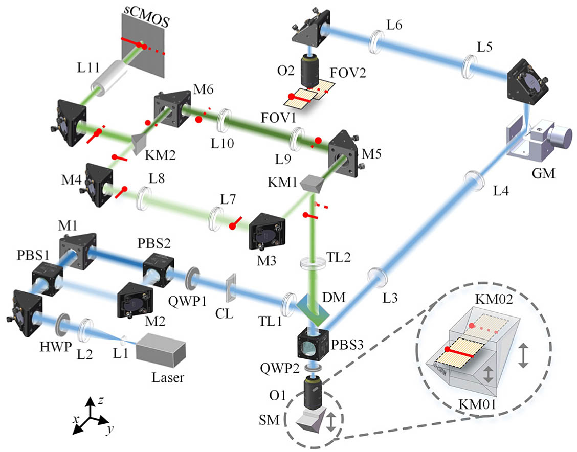
System configuration. The inset shows the enlarged view of the stepped mirror. The faint yellow plane represents the focal plane of O1. The positions of the stepped reflection surfaces were adjustable relative to the focal plane. Red lines and points represent two linear signals and their directions, respectively.

Figure 1.System configuration. The inset shows the enlarged view of the stepped mirror. The faint yellow plane represents the focal plane of O1. The positions of the stepped reflection surfaces were adjustable relative to the focal plane. Red lines and points represent two linear signals and their directions, respectively.

The back-pupil planes of objectives O1 and O2 (20XW/NA 1.0, XLUMPLFLN, Olympus, Tokyo, Japan) were conjugated by two telescope systems, L3 ( $f = 150 mm$ , AC254-150-A, Thorlabs) and L4 ( $f = 150 mm$ , AC254-150-A, Thorlabs) as well as L5 ( $f = 150 mm$ , AC254-150-A, Thorlabs) and L6 ( $f = 200 mm$ , AC254-200-A, Thorlabs). A one-axis galvanometer mirror (GM) (6240HM50A, 67124 H-1, Cambridge Technology, Bedford, MA, USA) was placed at the focal plane of L4 and L5 for fast linear beam scanning imaging. The SM was made by stitching two right-angle knife-edge mirrors KM01 and KM02 (MRAK25-G01, Thorlabs), as indicated in the inset of Fig. 1. Precisely moving one mirror up and down by a translation stage (N-565, Physik Instrumente, Karlsruhe, Germany) formed different step heights. Moving the entire SM by another translation stage (LNR25D/M, Thorlabs) achieved different remote focusing depths. Two linear beams, indicated by red lines with an endpoint, were focused at the focal plane of objective O1, as seen in the inset of Fig. 1; they were each reflected by the two surfaces, which were adjusted to above and below the focal plane, respectively, and then transmitted into the objective O2 and focused at two axial planes in the sample space. The excited fluorescent signals were transformed in the same way while returning, which were reflected by the SM again and focused at the same focal plane of O1.

The fluorescent signals were transmitted into the non-redundant detection part by a microscope composed of O1 and a tube lens TL2 ( $f = 180 mm$ , TTL180-A, Thorlabs) after the remote focusing part. The two parallel linear beams were focused at the imaging plane of TL2, which was also the edge plane of the knife-edge mirror KM1. They were reflected by the two surfaces of KM1 and were separated into two light paths. Two relay systems, L7 and L8 ( $f = 125 mm$ , AC254-125-A, Thorlabs), as well as L9 and L10 ( $f = 125 mm$ , AC254-125-A, Thorlabs), conjugated the linear beams to the edge plane of another knife-edge mirror KM2. Then, they were jointed into a collinear distribution with the heads connected by KM2. The emission light was transmitted through a $1 ∶ 1$ relay lens L11 ( $f = 45 mm$ , $f / 4$ , #45-760, Edmund, Barrington, USA) and an emission filter (AT525/30 m, Chroma), and was finally detected by the middle rows of a scientific complementary metal-oxide-semiconductor camera (sCMOS, ORCA-Flash 4.0, Hamamatsu Photonics K.K., Hamamatsu, Japan). The sample was fixed on a 3D translation stage (X axis, M-ILS250HA; Y axis, M-ILS100HA; Z axis, XMS50-S; Newport, Andover, USA) to control the imaging positions.

B. Principle

For a common microscope, two lines with an axial distance greater than the depth of field cannot be clearly imaged simultaneously. In comparison, we used an SM in the remote focusing system to generate and detect two lines at different axial depths with compensation for axial distance and spherical aberration. The two lines ( $u$ and $v$ ) focused on the nominal focal plane of O1, as shown in Fig. 2(a). The two surfaces of the SM were on either side of the focal plane of O1, and $d$ was the defocus distance of the upper surface of the SM. The reflected linear beams ( $u^{'}$ and $v^{'}$ ) can be regarded as emerging from the symmetrical plane about the mirror with the corresponding twice defocus distances and then carry the spherical aberration. According to the theory of remote focusing, the wavefront error at the pupil was odd-symmetric with the defocus position [22]. Thus, employing an opposing objective lens can counteract the wavefront error and translate the two lines to opposing positions in the remote space ( $u^{''}$ and $v^{''}$ ). We used a dry objective lens as O1 for conveniently adjusting the axial depths of the linear beams and used a water immersion objective lens as O2 to match the refractive index of the biological sample. The resolution did not deteriorate if the angular aperture was identical for both objective lenses. Thus, we used a telescope system that linked the pupil planes of the two objective lenses with a magnification equal to the ratio of the refraction indices of the immersion medium $n_{1}$ and $n_{2}$ of the objective lenses O1 and O2. The 3D magnification of the remote focusing system from the remote space to the sample space was the same as that of the telescope magnification: $M_{r} = n_{1} / n_{2} .$ (1)

Figure 2.Principle of stepped remote focusing and FOV-jointing. (a) Relative positions of the linear beams and the stepped mirror, as well as the geometric constraints of the distance between the linear beams and the step edge. Red, yellow, and pink points represent the linear beams perpendicular to the surface of the paper. (b) FOV-jointing module rearranges two parallel lines into a head-to-head line. The inset shows that the lateral interval between two linear signals is adjustable.

The axial interval in sample $l$ was proportional to the step height $h$ of the SM: $l = M_{r} \times H = \frac{n_{1}}{n_{2}} \times 2 \times h .$ (2)

To avoid clipping the beam by the step edge, the two linear beams must be away from the edge, as shown in Fig. 2(a). The distances between the linear beams and the step edge should meet the following conditions: ${\begin{cases} w_{1} \geq d \tan α_{eff}, \\ w_{2} \geq (2 h - d) \tan α_{eff}, \end{cases}$ (3)where $α_{eff}$ is the minimum semi-angular aperture of the two objectives. The lateral interval between the two FOVs in sample space $L$ is the distance between the two linear beams. Thus, given an imaging axial interval $l$ in the sample, $L$ satisfies the following requirement: $L = M_{r} (w_{1} + w_{2}) \geq M_{r} \times 2 h \tan α_{eff} = l \tan α_{eff} .$ (4)

Detecting two parallel separated lines by one camera also records useless data in the interval between the two lines and reduces the effective detection throughput and scanning speed. To solve this problem, we further combined the two lines into one collinear head-to-head line to avoid redundant detection. The main idea was to rotate the two lines by 90° in opposite directions. However, this was difficult to achieve with common rotating elements, such as the Dove prism. We proposed an FOV-jointing module consisting of two knife-edge mirrors and four plane mirrors, as shown in Fig. 2(b). We separated the two linear beams using KM1. After the reflections of M3 and M4, as well as M5 and M6, we recombined them with another knife-edge mirror KM2, which was rotated 90° compared to the first one. The two lines naturally became a collinear distribution, and the camera then detected them as a linear signal. Single-line detection avoids useless acquisition and allowed us to fully utilize the throughput of the camera and image in high-speed scanning. The maximum frame rate of the camera was 25.65 kHz with a minimal subarray width of eight lines, which was the fastest line rate of our system in this case.

The FOV-jointing module enabled the flexible adjustment of the lateral positions of the two FOVs before imaging according to specific experimental requirements. The lateral positions were controlled by changing the lateral interval, $L$ . Then, the vertical position of the detected linear signal on the camera was correspondingly changed. Vertically shifting the combination of TL2 and KM1 maintained the jointed linear signal at the middle of the camera, as indicated by the inset of Fig. 2(b). Owing to the infinite correction of objective O1, the adjustment had no influence on the imaging quality.

Detecting a single linear signal by the subarray of the camera also provided flexibility in controlling the optical sectioning [19 –21]. The subarray of the camera worked as a virtual confocal slit to inhibit the out-of-focus background. The narrower the slit width, the better the optical sectioning ability was. We could employ one line to generate confocal images with good optical sectioning, or multiple lines in time delay integration (TDI) to obtain a higher signal intensity with a slight sacrifice of optical sectioning. We could also choose suitable reconstruction algorithms and optical sectioning effects [19 –21] according to different experimental requirements in this work.

3. EXPERIMENTS AND RESULTS

A. Spatial Resolution and Axial Detection Range

To verify the imaging performance of our system, we measured the Strehl ratio and resolution in an axial range of 300 μm by imaging 200 nm fluorescent beads (FluoSpheresTM Carboxylate-Modified Microspheres, ThermoFisher, Waltham, MA, USA) in line confocal mode. The Strehl ratio is defined as the ratio of the maximum intensities of the images formed by a point source off and on the nominal focal plane [25]. This describes the deterioration of imaging due to aberrations. To avoid photobleaching, we scanned only seven layers with a $z$ step of 1 μm to determine the maximum pixel intensities. We scanned 21 layers with a $z$ step of 1 μm in another area to measure the 3D resolution. We repeated these measurements in a range of 150 μm above and below the nominal focal plane of the objective O2 with an interval of 50 μm. Figures 3(a) and 3(b) show the resolutions in the two FOVs, which maintained consistent at all axial positions in both FOVs, as shown in Fig. 3(c). The measured $x$ , $y$ , and $z$ resolutions were $0.50 \pm 0.05 μm$ , $0.57 \pm 0.05 μm$ , and $4.19 \pm 0.34 μm$ (mean $\pm$ s.d., beads number, $n = 5$ , and axial positions, $n = 7$ ), respectively. The axial $z$ resolution was slightly larger than the diffraction limit. This may have been caused by the absence of a coverslip under the coverslip-corrected objective O1 [26]. Figure 3(d) shows that the Strehl ratio was maintained above 80% for both FOVs in the axial range of $\pm 150 μm$ , indicating that the imaging quality was good [25]. The depth of the highest-intensity pixel was taken as the real focal plane. This was different from the focal plane calculated by the depth of the SM using Eq. (2) owing to the residual misalignment of the system. As the difference increased linearly with depth, we corrected Eq. (2) by multiplying by a correction coefficient of 1.01. After correction, the position offsets were close to zero, as shown in Fig. 3(e).

Figure 3.Resolutions and Strehl ratio measurements in an axial range of $\pm 150 μm$ . (a) and (b) Spatial resolutions of the two FOVs, respectively. Averaged pictures of beads are shown as corresponding insets at the top right corners. Pixel size, 0.244 μm in $x$ and $y$ as well as 1 μm in $z$ . (c) FWHM results. (d) Measured Strehl ratio. Standard deviations of five beads are shown as error bars. (e) Position offsets of the remote focal planes of the objective O2 in FOV1 and FOV2 at different depths before and after correction.

As the knife-edge planes of KM1 and KM2 and the detecting plane are conjugated, the two edges of the knife-edge mirrors show clearly on the camera, as shown in Fig. 4(a). This also is a critical alignment of the system. The edge of KM1 was shown horizontally as indicated by blue arrows. The two sides of the edge were shown on the left and right parts of the image, respectively. The edge of KM2 was shown vertically at the middle of the image, as indicated by the yellow arrow. We also adjust the two mirrors KM01 and KM02 of the SM in focus as indicated by red arrows. The area in the white square is enlarged in Fig. 4(b). The lateral interval between the two mirrors of the SM was about 5 μm. We moved KM01 10 μm down and kept KM02 still, and then we captured another image, as shown in Fig. 4(c). The edge of KM01 became blurred due to defocus as indicated by white arrow, while the edge of KM02 was still in focus. It indicates that our system enables to tune or scan the axial position of one FOV and fix another one.

Figure 4.Imaging the edges of the knife-edge mirrors of the FOV-jointing module and the stepped mirror. (a) Edges of KM1, KM2, KM01, and KM02 are shown clearly on the camera when they are conjugated and in focus. Scale bar, 50 μm. (b) Enlarged view of white square in (a). (c) Imaging the same area of (b) by moving KM01 10 μm down. Scale bar, 5 μm.

B. Optical Sectioning Ability

To measure the optical sectioning ability, we imaged a thin fluorescent sheet and a pollen grain. The fluorescent sheet was made by spreading the fluorescent bead solution directly onto a glass slide without dilution and waiting for it to dry. To measure the optical sectioning thickness, we scanned the sample in 29 layers with a $z$ step of 1.5 μm in line confocal mode. We chose a flat $11 \times 11$ pixels area of the fluorescent sheet and averaged the signal intensity. We calculated the FWHM of the change in the signal intensity with defocusing as the optical sectioning thickness. We repeated the measurement in a range of 150 μm above and below the nominal focal plane with an interval of 50 μm. We plotted the change in signal intensities with defocusing of both FOVs [Figs. 5(a) and 5(b)] and their FWHMs [Fig. 5(c)] at the seven axial positions. The results show that there was no significant difference in the optical sectioning ability at different depths for both FOVs.

Figure 5.Optical sectioning ability of the system. (a) and (b) Defocusing responses of thin fluorescent sheet in the line confocal mode of the two FOVs. (c) Line confocal optical sectioning thickness with a line width of 1 pixel. (d) Line confocal and (e) LiMo-reconstructed images of the same layer of a pollen grain at different remote focal positions in the two FOVs. Scale bar, 10 μm. Right column shows normalized intensity profiles along corresponding colored lines in the images.

We also imaged the same layer of a pollen grain at the seven axial positions in the sample space of O2 in two FOVs in the line confocal mode, as shown in Fig. 5(d). The imaging results remained consistent at different axial depths, whereas the background inhibitions in each image were poor. We reconstructed the optical sectioning images using the line illumination modulation (LiMo) algorithm [19] without extra components or multiple data acquisition, as shown in Fig. 5(e). As the sample was scanned through the line illumination, the in-focus sample was naturally modulated by different illumination intensities of Gaussian distribution, while the defocused sample was modulated by uniform illumination. Then, optical sectioning could be improved by extracting the in-focus signal with LiMo reconstruction. The following equation was used to reconstruct the optical sectioning signal $I_{LiMo}$ : $I_{LiMo} = 2 \sum_{k = 5}^{8} I_{k} - \sum_{k = 1}^{12} I_{k},$ (5)where $I_{k}$ represents the intensity of the $k$ th row image when the imaged line sample is modulated by the $k$ th line illumination intensity. The results demonstrate that the optical sectioning effect was greatly improved compared with the line confocal images. The normalized intensity profiles along the corresponding colored lines in the images are shown in the right column of Figs. 5(d) and 5(e). The details of the pollen imaged at different depths have similar definitions in both imaging modes, while LiMo reconstruction achieved better background inhibition and contrast. The results indicated that the signal intensity and optical sectioning had no significant deterioration in the axial range of 300 μm for both FOVs, and the optical sectioning effect could be flexibly chosen.

C. Dual-Plane Brownian Motion Imaging in Video Rate

To demonstrate the high imaging speed and adjustable FOV positions of our system, we observed Brownian motion in video rate by imaging an aqueous solution of 200 nm fluorescent beads in two planes. As shown in Fig. 6(a), we sandwiched three coverslips and placed the aqueous solution of fluorescent beads into two cracks between the coverslips. Thus, the Brownian motion of the beads was restricted to two layers. The axial interval was the thickness of the middle coverslip. In this case, we precisely adjusted the step height of the SM and found that the axial interval was 150 μm. The two FOVs were set 240 μm laterally apart. The frame rate was 24.5 Hz, and the size was $1024 \times 1024$ pixels in TDI mode. To track the motion of the beads, we extracted the centers of each bead and linked them in time sequences using the steps shown in Fig. 6(b). We first subtracted the offset of the camera and then discarded connected domains of less than eight pixels to eliminate salt-and-pepper noise. We then cross correlated the images with a Gaussian function, which was an analog of the system PSF, to smooth the intensity distribution of each bead. The peaks of the images were labeled as the centers of the beads. Then, we found the centers at previous time points and linked them with a straight line to plot the motion trajectories of the beads. At some time points, some beads flowed to the defocused planes and were difficult to extract in the image. We then found the beads at earlier time points and linked the centers. The trajectories of the Brownian motion of the beads in 2 s in FOV1 and FOV2 are shown in Figs. 6(c) and 6(d), respectively. The areas indicated by the white squares in Figs. 6(c) and 6(d) are enlarged in Figs. 6(e) and 6(f), respectively. A movie of these two layers of Brownian motion is shown in Visualization 1. Average speed of four beads in Figs. 6(e) and 6(f) was $8.21 \pm 0.36 μm / s$ (mean $\pm$ sem, $n = 4$ ). The motion trajectories of the bead in the right of Fig. 6(e) is close to a straight line, while the ones of other three beads are randomly curved. These results indicate our method is potentially capable of capturing the characteristics of cell motions, such as sperm motility measurement.

Figure 6.Video-rate imaging of two-layer Brownian motion of 200 nm fluorescent beads aqueous solution. (a) Sandwich structure of the sample. (b) Steps to track motion trajectories of the beads. (c) and (d) Trajectories of Brownian motions of the beads in FOV1 and FOV2. (e) and (f) are enlarged views of the areas indicated by the white squares in (c) and (d), respectively.

To demonstrate the flexibility in real-time imaging, we imaged another Brownian motion of double-layer fluorescent bead aqueous solution with an axial interval of 180 μm. We scanned axially 40 μm up in FOV1 at a speed of 0.015 mm/s and fixed FOV2 during acquiring video-rate images. A movie of the imaging results is shown in Visualization 2. It indicates that our system is also able to remotely scan imaging depths and acquire 3D images.

D. Dual-Plane Functional Imaging of a Zebrafish Brain in vivo

To demonstrate the potential of simultaneous imaging of biological activities in different planes, we recorded fluorescent images of spontaneous neural activities in two brain regions of a 7-day-old transgenic zebrafish in elavl3:H2B-GCaMP6f line (Misha Ahrens, HHMI, Ashburn, Virginia, USA) in vivo. The experiment was approved by the Institutional Animal Ethics Committee of Huazhong University of Science and Technology. The sample was fixed in 1.2% low-melting-point agarose. We chose to simultaneously image the optic tectum and hindbrain, indicated by yellow rectangles in the inset of Fig. 7(a). The two FOVs of $250 μm \times 250 μm$ were 10 μm and 60 μm under the brain surface with a lateral interval of 130 μm. The exposure time was set to 0.95 ms/line. The frame rate was set to 1 Hz, which is the typical time for the dynamics of zebrafish neural activity. To acquire more signals, we integrated 14 lines in TDI mode. We recorded the image sequences of both FOVs in 240 s, as shown in Visualization 3. The MIPs of the imaging sequences of FOV1 and FOV2 are shown in Figs. 7(a) and 7(b), respectively. We found 95 neurons in the FOV1 and 55 neurons in the FOV2 with spontaneous fluorescence intensity fluctuation, as indicated by white squares and colored circles in Figs. 7(a) and 7(b), respectively. First, we aligned the images to eliminate the mismatch due to residual motion. Then, we linearly fitted the no-activity signals as a base and calculated the relative fluorescence intensity changes ( $Δ F / F$ ) as calcium signal traces. We chose five typical neurons in Figs. 7(a) and 7(b) and profiled their activity signals, as shown in Figs. 7(c) and 7(d), respectively. Some oscillations in the optic tectum and hindbrain were synchronous, whereas others were not. To verify the flexibility of the optical sectioning of our system, we also performed imaging at another position in 14-line detections and reconstructed its images using TDI and LiMo modes, as shown in Figs. 7(e) and 7(f), respectively. Then, we removed the CL and captured the same sample in wide-field mode, as shown in Fig. 7(g). We can hardly distinguish the cell bodies in the wide-field image. In contrast, both TDI and LiMo inhibited the background fluorescence better than the wide-field mode, and we could identify cell bodies in the images more easily. Compared with the TDI mode, the LiMo image has a lower background and fewer cell numbers owing to the thinner optical sectioning. This indicates that we should choose a suitable optical sectioning mode according to different experimental requirements. If the signals of interest are exactly located at the focal plane, thin optical sectioning, such as LiMo, is more appropriate to exclude out-of-focus interference. If acquiring more signals at the focal plane and its vicinity in the FOV is more important, the TDI mode can be used with little sacrifice of optical sectioning. Figure 7(h) further demonstrates the differences among the three imaging modes. The figure shows the intensity profiles of the two cell bodies indicated by the corresponding colored lines in the TDI, LiMo, and wide-field images. Although we can distinguish the left cell from all three images, it is the most difficult in the wide-field image because of its high background. The right cell in the TDI image appears dim in the LiMo image, indicating that the cell is out of focus. It also cannot be identified in the wide-field image. The optic tectum is the visual center, while the neural activities in the hindbrain reflect motorial behavior. These results indicate that our method is potentially capable of studying the simultaneous visual and motorial responses under specific visual stimulus and their functional correlation. In addition, the maximum axial imaging range of our method is capable of covering the whole zebrafish brain. Therefore, we can potentially expand the imaging range to other interested brain areas and study their specific functional correlations.

Figure 7.Simultaneous dual-plane functional imaging of a transgenic zebrafish brain in vivo. (a) and (b) MIPs of image sequences acquired in 240 s in two FOVs. Inset in (a) indicates that the two FOVs focus in optic tectum and hindbrain, respectively. White squares and colored circles represent the neurons with spontaneous activities. (c) and (d) Spontaneous fluctuations of neural cells marked by corresponding colored circles in (a) and (b), respectively. (e)–(g) Images of the same sample in TDI, LiMo, and wide-field modes. (h) Normalized intensity profiles along corresponding colored lines in (e)–(g).

4. CONCLUSION

We demonstrated a flexible, video-rate, and spherical aberration-compensated axial dual-line scanning imaging method. We used a remote-stepped reflection to generate and detect dual lines with compensation for spherical aberration. It allows simultaneous imaging of dual planes in a large axial range of 300 μm. Furthermore, we proposed an FOV-jointing module to rearrange the two lines into a head-to-head line to avoid redundant acquisition and achieve video-rate imaging. The FOV-jointing module also allows the flexible adjustment of the lateral positions of the FOVs. The subarray detection of a single linear signal by the camera makes it easy to cooperate with different line scanning optical sectioning imaging modalities and algorithms according to the experimental requirements. This dual-plane imaging method has the advantages of video rate, optical sectioning defocus-aberration compensation, and adjustability of optical sectioning and FOV positions.

Compared with existing parallel dual-plane imaging, our method allows a larger range of the axial imaging positions, and the flexible adjustments of the lateral positions of the FOVs before imaging and their axial positions during imaging. The speed is high enough to image biological processes in vivo. It allows us to study relations of neural activities in different areas in a wide range. Our method has no compromise in resolution, optical sectioning, or signal intensity compared with traditional line scanning microscopy. The optical sectioning can also be flexibly adjusted in various experiments. It allows us to achieve imaging of high resolution and thin optical sectioning for fine structures and also achieve thick optical sectioning for sparse samples. It can also realize imaging in stage scanning by moving the sample with unlimited sizes of FOVs.

In theory, this method would simultaneously detect more planes in the future by employing a multi-layer SM and a group of multiple FOV-jointing modules. It is possible to make the mirrors with multiple steps by means of photolithography [27] for multi-layer remote focusing. On the other hand, the modular design of the FOV-jointing allows us to expand the number of parallel lines that can be detected simultaneously by connecting multiple FOV-jointing modules in series. Thus, the number of lines that can be rearranged to one line is the power of the FOV-jointing module number of 2. For example, we can use four modules to reorganize 16 lines into one line. Sharing one camera is a more compact and feasible approach for integrating more channels compared with the multi-detector scheme. Therefore, the convenience of our method potentially becomes more noticeable as the number of planes increases. We only achieved 24.5 Hz with two planes in the current system owing to the limited transmission bandwidth of the camera. The throughput of our system could be further improved by changing it to other cameras with a higher line rate and longer line-array pixels. For example, a line scan camera (ML-HM-16k30H-00-R, Teledyne DALSA, Waterloo, ON, Canada) has $16,384 \times 4$ pixels and operates at 300 kHz, potentially allowing for the simultaneous imaging of 16 planes with a frame rate of 293 Hz. The remote focusing design in our system also permits us to scan imaging depths remotely. It provides the potential of acquiring video-rate multi-volume images by fast scanning a lightweight SM [28]. By combining it with two-photon microscopy, we could extend the potential application of simultaneously detecting multi-plane biological activities to highly scattering samples such as rodent animal models [29]. The FOV-jointing module can also translate two parallel lines at different axial planes to a single plane by controlling the relay systems and then rearrange them into a collinear line. In addition, tissue aberration in deep tissue may be further compensated with adaptive optics to expand effective imaging depth [22]. Thus, the proposed method will be particularly attractive in large-axial-range multi-plane imaging and potentially facilitates biological study in 3D in vivo.

Acknowledgment

Acknowledgment. The authors thank Dr. JiuLin Du, Miss. Jiwen Bu, and Dr. Ling Fu for providing the help with zebrafish experiments.

References

[1] N. Ji, J. Freeman, S. L. Smith. Technologies for imaging neural activity in large volumes. Nat. Neurosci., 19, 1154-1164(2016).

[2] R. Lu, W. Sun, Y. Liang, A. Kerlin, J. Bierfeld, J. D. Seelig, D. E. Wilson, B. Scholl, B. Mohar, M. Tanimoto, M. Koyama, D. Fitzpatrick, M. B. Orger, N. Ji. Video-rate volumetric functional imaging of the brain at synaptic resolution. Nat. Neurosci., 20, 620-628(2017).

[3] W. Yang, J. E. Miller, L. Carrillo-Reid, E. Pnevmatikakis, L. Paninski, R. Yuste, D. S. Peterka. Simultaneous multi-plane imaging of neural circuits. Neuron, 89, 269-284(2016).

[4] S. R. Pavani, M. A. Thompson, J. S. Biteen, S. J. Lord, N. Liu, R. J. Twieg, R. Piestun, W. E. Moerner. Three-dimensional, single-molecule fluorescence imaging beyond the diffraction limit by using a double-helix point spread function. Proc. Natl. Acad. Sci. USA, 106, 2995-2999(2009).

[5] F. Xu, D. Ma, K. P. MacPherson, S. Liu, Y. Bu, Y. Wang, Y. Tang, C. Bi, T. Kwok, A. A. Chubykin, P. Yin, S. Calve, G. E. Landreth, F. Huang. Three-dimensional nanoscopy of whole cells and tissues with in situ point spread function retrieval. Nat. Methods, 17, 531-540(2020).

[6] W. J. Shain, N. A. Vickers, J. Li, X. Han, T. Bifano, J. Mertz. Axial localization with modulated-illumination extended-depth-of-field microscopy. Biomed. Opt. Express, 9, 1771-1782(2018).

[7] A. Song, A. S. Charles, S. A. Koay, J. L. Gauthier, S. Y. Thiberge, J. W. Pillow, D. W. Tank. Volumetric two-photon imaging of neurons using stereoscopy (vTwINS). Nat. Methods, 14, 420-426(2017).

[8] A. Cheng, J. T. Goncalves, P. Golshani, K. Arisaka, C. Portera-Cailliau. Simultaneous two-photon calcium imaging at different depths with spatiotemporal multiplexing. Nat. Methods, 8, 139-142(2011).

[9] D. R. Beaulieu, I. G. Davison, K. Kilic, T. G. Bifano, J. Mertz. Simultaneous multiplane imaging with reverberation two-photon microscopy. Nat. Methods, 17, 283-286(2020).

[10] P. Prabhat, S. Ram, E. S. Ward, R. J. Ober. Simultaneous imaging of different focal planes in fluorescence microscopy for the study of cellular dynamics in three dimensions. IEEE Trans. Nanobiosci., 3, 237-242(2004).

[11] A. Badon, S. Bensussen, H. J. Gritton, M. R. Awal, C. V. Gabel, X. Han, J. Mertz. Video-rate large-scale imaging with multi-Z confocal microscopy. Optica, 6, 389-395(2019).

[12] A. Descloux, K. S. Grußmayer, E. Bostan, T. Lukes, A. Bouwens, A. Sharipov, S. Geissbuehler, A. L. Mahul-Mellier, H. A. Lashuel, M. Leutenegger, T. Lasser. Combined multi-plane phase retrieval and super-resolution optical fluctuation imaging for 4D cell microscopy. Nat. Photonics, 12, 165-172(2018).

[13] S. Xiao, H. Gritton, H.-A. Tseng, D. Zemel, X. Han, J. Mertz. High-contrast multifocus microscopy with a single camera and z-splitter prism. Optica, 7, 1477-1486(2020).

[14] S. Abrahamsson, J. Chen, B. Hajj, S. Stallinga, A. Y. Katsov, J. Wisniewski, G. Mizuguchi, P. Soule, F. Mueller, C. D. Darzacq, X. Darzacq, C. Wu, C. I. Bargmann, D. A. Agard, M. Dahan, M. G. Gustafsson. Fast multicolor 3D imaging using aberration-corrected multifocus microscopy. Nat. Methods, 10, 60-63(2013).

[15] P. A. Dalgarno, H. I. C. Dalgarno, A. Putoud, R. Lambert, L. Paterson, D. C. Logan, D. P. Towers, R. J. Warburton, A. H. Greenaway. Multiplane imaging and three dimensional nanoscale particle tracking in biological microscopy. Opt. Express, 18, 877-884(2010).

[16] C.-M. Chia, H.-C. Wang, J. A. Yeh, D. Bhattacharya, Y. Luo. Multiplexed holographic non-axial-scanning slit confocal fluorescence microscopy. Opt. Express, 26, 14288-14294(2018).

[17] L. V. D. Graaff, G. J. L. H. van Leendersc, F. Boyaval, S. Stallinga. Multi-line fluorescence scanning microscope for multi-focal imaging with unlimited field of view. Biomed. Opt. Express, 10, 6313-6339(2019).

[18] J.-M. Tsang, H. J. Gritton, S. L. Das, T. D. Weber, C. S. Chen, X. Han, J. Mertz. Fast, multiplane line-scan confocal microscopy using axially distributed slits. Biomed. Opt. Express, 12, 1339-1350(2021).

[19] Q. Zhong, A. Li, R. Jin, D. Zhang, X. Li, X. Jia, Z. Ding, P. Luo, C. Zhou, C. Jiang, Z. Feng, Z. Zhang, H. Gong, J. Yuan, Q. Luo. High-definition imaging using line-illumination modulation microscopy. Nat. Methods, 18, 309-315(2021).

[20] Q. Zhong, C. Jiang, D. Zhang, S. Chen, R. Jin, H. Gong, J. Yuan. High-throughput optical sectioning via line-scanning imaging with digital structured modulation. Opt. Lett., 46, 504-507(2021).

[21] W. Qiao, R. Jin, T. Luo, Y. Li, G. Fan, Q. Luo, J. Yuan. Single-scan HiLo with line-illumination strategy for optical section imaging of thick tissues. Biomed. Opt. Express, 12, 2373-2383(2021).

[22] Y. Yang, W. Chen, J. L. Fan, N. Ji. Adaptive optics enables aberration-free single-objective remote focusing for two-photon fluorescence microscopy. Biomed. Opt. Express, 12, 354-366(2021).

[23] E. J. Botcherby, R. Juškaitis, M. J. Booth, T. Wilson. An optical technique for remote focusing in microscopy. Opt. Commun., 281, 880-887(2008).

[24] E. J. Botcherby, M. J. Booth, R. Juškaitis, T. Wilson. Real-time slit scanning microscopy in the meridional plane. Opt. Lett., 34, 1504-1506(2009).

[25] V. N. Mahajan. Strehl ratio for primary aberrations: some analytical results for circular and annular pupils. J. Opt. Soc. Am., 72, 1258-1266(1982).

[26] S. Mohanan, A. D. Corbett. Sensitivity of remote focusing microscopes to magnification mismatch. J. Microsc..

[27] T. Chakraborty, B. Chen, S. Daetwyler, B. J. Chang, O. Vanderpoorten, E. Sapoznik, C. F. Kaminski, T. P. J. Knowles, K. M. Dean, R. Fiolka. Converting lateral scanning into axial focusing to speed up three-dimensional microscopy. Light Sci. Appl., 9, 165(2020).

[28] E. J. Botcherby, C. W. Smith, M. M. Kohl, D. Débarre, M. J. Booth, R. Juškaitis, O. Paulsen, T. Wilson. Aberration-free three-dimensional multiphoton imaging of neuronal activity at kHz rates. Proc. Natl. Acad. Sci. USA, 109, 2919-2924(2012).

[29] Y. Xue, J. R. Boivin, D. N. Wadduwage, J. K. Park, E. Nedivi, P. T. C. So. Multiline orthogonal scanning temporal focusing (mosTF) microscopy for scattering reduction in high-speed in vivo brain imaging(2019).