With the further intensification of human activities, their interference with the ecosystem affects the quality of biological habitats and leads to the degradation of biodiversity. Currently, with the rapid development of China's urbanization, the sharp expansion of impervious grounds is significantly influencing regional habitat quality, with considerable challenges for biodiversity protection (Brandt et al., 2014; Yuan et al., 2017). Habitat quality refers to the ability of an ecological system to provide living conditions that are suitable for the sustainable development of individuals and populations, reflecting the status of regional biodiversity to some extent (Fellman et al., 2015; Hillard et al., 2017). Habitat quality also reflects the health status of an ecosystem and plays an important role in maintaining the biodiversity level (Dominique et al., 2018; Barbara and Stefan, 2018). In the past few decades, human activities have led to habitat disappearance and fragmentation as well as to habitat quality degeneration, with serious consequences for biodiversity and human welfare (Haddad et al., 2015; Newbold et al., 2015). Land use change reflects the intensity of human activities, which is the most important threat factor of habitat quality (Otto et al., 2016; Lohse et al., 2008). In this sense, it is of great significance for regional biodiversity conservation and the sustainable use of land resources to explore changes in regional habitat quality and to analyze the spatial distribution characteristics of habitat quality degradation based on land use change.

In the field of land use spatial pattern reconstruction, the most representative research achievements are the establishment of the global history environment dataset (HYDE) (Goldewijk et al., 2010) and the global land use dataset (SAGE) (Ramankutty and Foley, 2010). Generally, spatial land use pattern reconstruction is as follows: In the case of certain proposed reconstruction hypotheses, the historical land quantity is first reconstructed, and subsequently, the conversion rules, distribution methods, and constraint conditions are identified via geographical spatial analysis; finally, the historical land quantity is spatialized to acquire the land use spatial dataset (Yang et al., 2015; Long et al., 2014; Zhu et al., 2012). The historical land quantity can be reconstructed mainly by integrating the overall statistical data from various kinds of historical sources and by combining them with certain assumptions to estimate land quantity at certain historical periods. Land use spatial reconstruction methods can mainly be divided into two categories: the restoration method, based on historical records, and the reconstruction method, based on geographical spatial models (Yang et al., 2016). Since there is a limited quantity of historical data available, which are difficult to access, existing research on land use spatial reconstruction is given priority to the reconstruction method based on geographical spatial models. For example, Jiang et al. (2015) and He et al. (2015), using spatial grids as the reconstruction basic unit, adopted the cultivated land reclamation tendency index and the land reclamation suitability as the distribution method to reconstruct the cultivated land spatial pattern on the Songnen Plain in the late Qing Dynasty and the gridding forest coverage conditions of China over 1700-2000. Similarly, Yang et al. (2016) reconstructed the spatial distribution of cultivated land in Shandong Province between 1661 and 1952 by using the multi-agent model, while Long et al. (2014) reconstructed the historical spatial pattern of cultivated land in Jiangsu Province via CA. Generally, because of the focus on cultivated land protection and food production, studies on the reconstruction of land use spatial patterns mostly considered a certain land use type, such as cultivated land. However, there is little research on the comprehensive reconstruction of all land use types from the ecological perspective, not to mention regional habitat quality analysis on the basis of land use spatial pattern reconstruction.

Current research on habitat quality mainly concentrates on two aspects: habitat quality assessment on individual species (Tang et al., 2016; Zhang et al., 2014) and regional habitat quality assessment (Zhong and Wang, 2017; Wu et al., 2015). Habitat quality assessment on individual species first determines the distribution scope and characteristics of the habitat based on the habitat requirements of living beings and their matching relations with the local natural environment (Zhang et al., 2014) and then constructs the assessment index system to comprehensively assess habitat quality. For instance, habitat quality assessments on the white stork (Li and Bai, 2006), egrets (Wu and Lian, 2018), pandas (Zhang et al., 2014), Helan Mountain blue sheep (Liu et al., 2013), and the Qinling Mountain System musk deer (Luo et al., 2011) are all assessments on individual species. Nevertheless, in this method, data acquisition is expensive, and this method is not suitable for comprehensive, large-scale assessment studies. Hence, related studies are usually carried out in small-scale nature reserves or watersheds. Regional habitat quality assessment mostly adopts the InVEST model to conduct multi-scale quantitative habitat quality assessments. This model was jointly developed by Stanford University, the Nature Conservancy, and the World Wide Fund for Nature (Tallis et al., 2013) and can be used for quantitative analysis of a variety of ecosystem service functions such as habitat quality (Lin et al., 2017), soil conservation function (Li et al., 2017), carbon reserves (Pechanec et al., 2017), water yield (Redhead et al., 2016), and water purification (Wang et al., 2017), and the analysis results can be expressed in the form of thematic maps. By using the InVEST model, Sallustio et al. (2017) and Terrado et al. (2016) respectively assessed the habitat quality of nature reserves and the watershed habitat quality under different scenarios of natural conservation planning in Italy. Similarly, Li et al. (2018) combined the InVEST model with the SLEUTH model and simulated the urban expansion situation based on habitat quality protection. Based on the InVEST model, Chu et al. (2015), Liu et al. (2018), and Deng et al. (2018) respectively investigated the quantitative relations between landscape pattern and habitat quality in coastal zones, the habitat quality of the transitional zone of three nature reserves, and the influences of urban expansion in the Beijing-Tianjin-Hebei region on the spatial-temporal pattern of habitat quality.

Such studies complement the used study areas for regional habitat quality assessment, such as nature reserves, coastal zones, watershed units, and rapid urbanization areas, thereby promoting the development of habitat quality assessment. However, limited by the inaccessibility of land use data in specific historical periods or under future scenarios, these authors mainly focused on exploring the present situation of regional habitat quality and the spatial-temporal variation of habitat quality, but largely neglected the spatial simulation of habitat quality for certain historical or future periods. Hence, regional habitat quality assessment based on the reconstruction of spatial land use patterns at certain historical periods can acquire the evolution rules of habitat quality on a longer time scale, provide long time-series data support for habitat quality protection and a scientific basis for habitat quality management.

This paper aims to inversely deduce land use spatial patterns at certain historical periods by the CA-Markov model when historical data are lacking and to reconstruct the spatial pattern of regional habitat quality at certain historical periods by using the InVEST model. On this basis, the spatial-temporal variation of habitat quality in the study area against the background of rapid economic development since China’s reform and opening-up in 1978 was recalled. Our work provides a reference for regional biodiversity conservation and regional ecological development, long time-series data support for regional eco-environmental studies, and new means for recalling the historical habitat quality situation and predicting the future habitat quality situation.

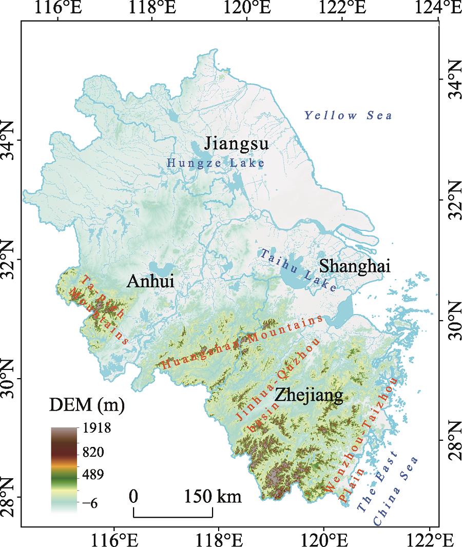
The Pan-Yangtze River Delta region is located in eastern China within the scope of 114°54'-122°12'E and 27°09'-35°20'N. It includes one municipality and three provinces, i.e., Shanghai, Zhejiang, Jiangsu, and Anhui (Figure 1). The climate is subtropical humid monsoon climate, with warm winters and cool summers; there are four distinct seasons and abundant rain. The terrain is high in the south and low in the north, and the landforms are mainly plains, mountains, and hills. This region covers an area of about 359,000 km². The population of permanent residents increases yearly and reached 223 million capita in 2017. Population aggregation promotes the economic development and urban expansion. According to statistical data, from 2010 to 2016, the GDP increased by 1.8 times to 17.72 trillion yuan, with an average annual increase rate of 10.30%. The urban area also increases constantly, with an average annual growth rate of 2.28%. Rapid economic development and urban expansion lead to the conversion of regional land use types, regional habitat segmentation, and increased habitat fragmentation, thus resulting in the degradation of habitat quality.

We obtained land use data for 2000, 2005, and 2010 from the Resources and Environment Data Sharing Center of the Chinese Academy of Sciences. There were six land use types, including cultivated land, forest land, grassland, water area, construction land, and unused land. Social and economic data were obtained in the form of 1-km grid interpolation data of China’s GDP and population in 2010 from the Resources and Environment Data Sharing Center of the Chinese Academy of Sciences. The digital elevation model (DEM) data were obtained from the SRTMDEM original elevation map of 90 m on the geospatial data cloud, and the slope and aspect data were extracted from the downloaded DEM data. Climate data were represented by the annual average air temperature and rainfall data downloaded from the China Meteorological Data Sharing Network. The cell size in the CA model of this study was 1 km², and the above data were all processed into grid data of 1 km × 1 km.

2.3.1 CA-Markov model

The Markov model can predict the status of a certain event in the following period based on its status in the current period. The model is a long-term prediction method, and the key of using it is to determine the conversion probability of the event (Anderson and Goodman, 1957). In the Markov process, land use change can be expressed as follows (Zhou et al., 2018):

where X(t+1) represents the state of the random event at time t + 1, namely the prediction results by the Markov model; X(t) represents the state of the random event at time t; P is the conversion probability matrix, representing the probability of the conversion between different states of the random event.

The CA model is a complex dynamic model and composed of cell space, cell unit size, states collection, and neighborhood scope. In the CA model, it is important to determine the cell state conversion rules (Li, 2007); the model can be expressed as follows (Zhou et al., 2018):

where S is the limited, discrete states collection of the cell; f is the state conversion rule; N is the neighborhood scope of the cell.

Both models are widely used in the simulation and prediction of land use changes (Lv et al., 2017; Chen et al., 2017). However, the Markov model can only predict the land use quantity, while the CA model ignores the influencing factors. We can overcome these limitations by combining these two models, namely by making full use of the strong spatial simulation ability of the CA model and the long-term prediction ability of the Markov model (Pan et al., 2018; Hu et al., 2018).

In this study, we used the two-dimensional cellular space, and the grid type in the cellular space was square grid. The domain of the cell was the 5×5 extendable Moore domain. Land use conversion was based on the adaptability of various land use types in the adaptability maps, and the land use type with the strongest adaptability was chosen for conversion. When running the model, the number of iterations was set according to the predictionuration. For example, if the prediction interval was 5 years, the number of iterations was set at 5. When we used the Markov model to predict the future land use quantity, the conversion quantity of various land use types was computed in the running process of the model. When the conversion quantity achieved the predicted quantity of the Markov model, the model was stopped, and the reconstruction of the spatial land use pattern was completed. Compared with traditional predictions on future land use scenarios, the selection of driving forces in historical land use simulation places more emphasis on the driving force factors in terms of natural conditions.

2.3.2 Kappa consistency check

The Kappa consistency check is used to measure the precision of the prediction results from a certain model. After the completion of the consistency check, the Kappa coefficient can be acquired, which is an indicator to measure the precision of prediction results. The Kappa consistency check is based on the confusion matrix, and the calculation formula is as follows:

where Kappa is the calculated test precision; P_o and P_e are the overall simulation precision and the theoretical simulation precision, respectively;${{a}_{1}},{{a}_{2}},\cdots ,{{a}_{c}}$ are the percentages of correct simulations for each land use type;$\text{ }\!\!~\!\!\text{ }{{b}_{1}},{{b}_{2}},\cdots ,{{b}_{c}}$ are the predicted percentages of each land use type;${{d}_{1}},{{d}_{2}},\cdots ,{{d}_{c}}$ are the actual percentages of each land use type. If the Kappa coefficient varies within 0-0.20, the precision of simulation result is very low; if it varies within 0.20-0.40, the simulation precision is low; if it varies within 0.40-0.60, the simulation precision is medium; if it varies within 0.60-0.80, the simulation precision is high; if it varies within 0.80-1.00, the simulation precision is very high.

2.3.3 Habitat quality model

We used the habitat quality module of the InVEST model to assess habitat quality. The assessment by this module reflects the influences of human activities on the eco-environment. The stronger the intensity of human activities, the greater the threat to the habitat and the lower the habitat quality and the biodiversity level in this region; on the contrary, the higher the habitat quality, the lower the interferences from human activities and the higher the biodiversity level in this region (Xie et al., 2018). Our study combines the sensitivity of different land use types to threat factors and the intensity of external threats, computes the degradation degree of habitat quality, and further calculates habitat quality, using the following equations (Liu et al., 2017):

where${{\omega }_{r}}$is the weight of different threat factors; r_y is the intensity of the threat factor; ${{\beta }_{x}}$ is the anti-interference level of habitat; S_ir is the relative sensitivity degree of different habitats to different threat factors; r is the habitat threat factor; y is the grid in the threat factor r; d_xy is the distance between grid x and grid y; ${{d}_{r\max }}$is the influencing scope of the threat factor r. The habitat degradation degree varies between 0 and 1; the higher the value, the higher the habitat degradation degree.

The calculation formula of habitat quality is as follows (Liu et al., 2017):

where Q_xj is the habitat quality of grid x in land use type j; D_xj is the habitat degradation degree, which represents the habitat degradation degree of grid x in land use type j; H_j is the habitat adaptability of grid x in land use type j; k is a half-saturation constant. The habitat quality value is between 0 and 1; the higher the value, the higher the habitat quality.

Based on the comprehensive consideration of the situation of the study area, relevant research results, and expert opinions, we selected cultivated land, construction land, and unused land as threat factors. The parameters of threat factors that need to be set include the longest threat distance, weight, and spatial decay type; the sensitivities of land use types to threat factors need to set the parameters of the habitat suitability of each land use type and the sensitivity of each land use type to the threat factor. The above parameters were set after referring to the user manual of the InVEST model (Tallis et al., 2013), previous results (Zhong and Wang, 2017; Wu et al., 2015; Liu et al., 2017), and expert opinions. The specific parameter settings are listed in Tables 1 and 2.

2.3.4 Habitat quality change rate and habitat degradation degree change rate

The habitat quality change rate refers to the change percentage of regional habitat quality at the end of a certain period relative to that at the beginning of the period. The habitat degradation degree change rate describes the change rate of habitat degradation degree at the end and the beginning of a certain period. Both rates have the same calculation formula:

where v denotes the change rate of habitat quality or habitat degradation degree; ${{P}_{{{t}_{0}}}}$and ${{P}_{{{t}_{1}}}}$ are the values of habitat quality (or habitat degradation degree) at the beginning and the end of a certain period, respectively. When the value of v is negative, the habitat quality or habitat degradation degree declines and vice versa.

We selected elevation, slope, aspect, GDP, population, temperature, precipitation, river distance, urban distance, and coastline distance, a total of 10 indicators, as the driving force factors of land use changes. Via logistical analysis, the land adaptability atlas was drawn, using the following equation:

where P_i represents the probability of the i-th land use type appearing in each grid in the grid diagram; x₁, x₂, …, xn represents the driving force factors that affect the conversion of land use types (Zhou et al., 2018).

The ROC test method was adopted to test the logistical analysis results. It represents a quantitative measurement method applied to the model precision test of the model that generates the land use adaptability graphs (Jr and Schneider, 2001). The test values of the method are between 0 and 1; the closer the ROC value is to 1.0, the more ideal the fitting results. When ROC≥0.9, the fitting results have a higher precision; when 0.9>ROC≥0.7, the fitting results have a certain precision; when 0.7 > ROC > 0.5, the fitting results have a lower precision; when ROC = 0.5, the fitting method is completely ineffective; when ROC < 0.5, the fitting results do not conform to the real situation. Generally, fitting results are considered good when ROC > 0.7. Table 3 provides the coefficients of the logistical regression results and the test results; all ROC values in the table are greater than 0.8.

According to the land use data for 2010 and 2005, we obtained the land use conversion matrix. Via the CA-Markov module in IDRISI, we acquired six periods of land use data for 1975, 1980, 1985, 1990, 1995, and 2000. By using the real land use data for 2000 and the simulated land use data for the same year, we conducted the model simulation precision test. Figures 2 and 3 show the real land use maps and the simulated land use maps by CA-Markov simulation, respectively, for 2000, 2005, and 2010.

The simulation results were tested by using the Kappa consistency check, and the predicted results were tested via the CROSSTAB module in IDRISI. First, the confusion matrix was generated, and then, according to Eqs. (3)-(5), we obtained the overall simulation precision, the theoretical simulation precision, and the Kappa coefficients of 0.93, 0.42, and 0.88 respectively. These results indicate that the CA-Markov model has a high simulation precision, and that the simulation results can support the reconstruction simulation of habitat quality by the InVEST model. In the seven periods (from 1975 to 2010), in the study area, the area of cultivated land decreased constantly, with change rates of 0.13%, 0.22%, 0.45%, 0.85%, 2.39%, 2.23%, and 7.10%. The area of forest land showed an overall decreasing trend; except for a slight increase by 1.96% between 2000 and 2005, the change rates in the other periods were 0.40%, 0.46%, 0.57%, 0.72%, 3.95%, and 1.25%. The areas of grassland and construction land both showed an increasing trend. The grassland area increased by 1.27%, 1.72%, 2.31%, 2.86%, 2.785, 2.715, and 3.18%, while the construction area increased by 2.08%, 3.64%, 7.03%, 13.80%, 32.39%, 31.85%, and 64.28%. The water area only changed slightly. The area of unused land accounted for a small proportion of the total study area and only changed slightly.

The habitat quality module in the InVEST model was employed to reconstruct the spatial pattern of habitat quality, obtaining the spatial patterns of habitat degradation degree and habitat quality at eight periods in 2010, 2005, 2000, 1995, 1990, 1985, 1980, and 1975. Among these, the spatial patterns in 2010, 2005, and 2000 represent the assessment results based on existing monitoring data, while those for other periods represent the assessment results based on simulation reconstruction.

The habitat degradation degree varies between 0 and 1; the higher the value, the higher the habitat degradation degree. According to the computational results of the InVEST model, we obtained the average habitat degradation degree (Figure 4) and the spatial distribution of the habitat degradation degree (Figure 5) in the study area from 1975 to 2010. Subsequently, according to Eq. (10), we calculated the change rate of the habitat degradation degree. The results show that from 1975 to 2010, the habitat degradation degree in the study area increased constantly. From 2000 to 2005 and from 2005 to 2010, the habitat degradation degree increased by 3.53% and 7.30%, respectively. During the four periods from 1975 to 1995, the habitat degradation degree increased by 5.47%, 6.98%, 9.12%, and 12.32%, respectively, and the change rate of the degradation degree increased constantly, which was consistent with the actual change trend from 2000 to 2010. The above results show that during the period from 1975 to 2010, the intensity of human activities was enhanced, and their interference with the ecosystem was aggravated, leading to the gradual increase in habitat degradation.

4.1.1 Spatial-temporal variation of habitat degradation degree

According to Figure 5, in terms of the spatial distribution of habitat degradation, the high-value zones were mainly distributed in the core areas of regional economic development, such as Shanghai, the south of the stem stream of the Yangtze River (the section from Nanjing to Shanghai), and the Hangzhou Bay region. Other high-value zones were distributed in plains, basins, mountainous areas, rivers, and lakes, where the economy develops rapidly, such as the plains along the Yangtze River in Anhui Province (the stem stream of the Yangtze River from Awning to Maanshan), the Jinqu Basin in Zhejiang Province, the Dabie Mountain, the Huangshan Mountain, and the mountainous areas in southern Zhejiang Province, as well as Lake Taihu, Lake Hongze, and Lake Chaohu. Overall, zones with a high habitat degeneration were marginally distributed along the built-up areas, mountains, and lakes, with a circular structure. In contrast, zones with low habitat degradation presented a spatial distribution of ‘more in the north and less in the south’. Such low-value zones were mainly distributed in northwestern Anhui, eastern Jiangsu, and the mountainous areas of southern Zhejiang. Other low-value zones were surrounded by high-value zones, and the interiors of urban built-up areas, mountains, rivers, and lakes were all low-value zones. In terms of the spatial-temporal variation, the distribution of high-value zones changed only slightly from 1975 to 2010, but the number of plaques presented an increasing trend. The added plaques were mainly concentrated in Suzhou-Zhenjiang, the plains along the Yangtze River in Anhui, and the Jinqu Basin. Low-value zones were continuously segmented, and the plaques became more and more fragmented. Three kinds of low-value zones, namely built-up areas, rivers, and lakes, remained their original state.

The spatial variation in habitat degradation reflects the severity of regional habitat quality degradation. The distribution and variation of habitat degradation show that habitat quality is more likely to be destroyed in regions with higher economic development rates. In particular, urban expansion has significant destruction effects on habitats, and consequently, the high-value zones of habitat degradation are mainly distributed around urban built-up areas; at the same time, within these areas, habitat degradation remains low because of the serious initial degradation. In regions which are difficult to develop, such as mountains, rivers, and lakes, habitat quality basically remains constant. In the marginal areas of the above regions, although human activities have a low intensity, interferences are possible. As a result, the degradation in these marginal areas is lower, and the scope of these marginal areas is limited.

4.1.2 Variation characteristics of habitat degradation degree grades

According to the model assessment results, we graded the habitat degradation degrees in ArcGIS by the NBC (natural break-point classification) method into five grades (Figure 6), including no degradation (0), mild degradation (0-0.005), moderate degradation (0.005-0.015), high degradation (0.015-0.03), and severe degradation (0.03-Max). Spatially, the habitat degradation degree showed a trend of layered progressive distribution. At the center of the layers, habitat degradation was absent or mild. From the center to the outside, degradation can be divided into two types: a progressive increasing trend from moderate degradation over high to severe degradation and a progressive decreasing trend from severe degradation over high to moderate degradation.

The center of the first type of the layered structure is located in mountainous areas, nature reserves, or lakes, which are difficult to develop and use and therefore hardly affected by human activities. As a result, the center of the layered structure is not or only mildly degraded. The closer the regions are to the center, the lower the interference of human activities and the lower the habitat degradation degree grade. In the marginal regions of the Dabie Mountain, the Huangshan Mountain, the mountainous areas in southern Zhejiang Province, Lake Taihu, Lake Hongze, and Lake Chaohu, the habitat degradation degree grade presents this type of layered structure. In these marginal regions, human activities are frequent, but the internal regions are not suitable for large-scale agricultural production and economic development. Consequently, the intensity of human activities is low in the internal regions, with neglectable interferences. Hence, the habitat degradation degree in the marginal regions presents an increasing trend.

The center of the second type of layered structure is located in urban areas which are difficult to change in terms of land cover type, and the habitat degradation degree grade is therefore low. The closer the regions are to the built-up areas, the more significantly they are affected by urban expansion and the higher the habitat degradation degree grade due to changes in land cover types. (1) Shanghai-Suzhou-Wuxi-Zhenjiang-Nanjing on-axis regions and their surrounding regions as well as the Hangzhou-Ningbo on-axis regions have the most significant second-type layered structure. These regions are located in the core development region of the Pan-Yangtze River Delta region, with rapid urban and economic growth. Hence, land use changes are significant, and the intensity of human activities in these regions is higher than in other regions of the study area. As a result, the habitat degradation degree in these regions is higher than in other regions. (2) Hefei, Xuzhou, Lianyungang, Huai’an, Yancheng, Jinqu Basin of central Zhejiang, Wentai Plain of southeastern Zhejiang, and the north of Hangzhou Bay area also present such type of layered structure. Hefei is the capital city of Anhui Province, and Xuzhou, Lianyungang, Huai’an, and Yancheng are important cities of Jiangsu Province. They are hotspots of regional economic growth and development, with rapid urban expansion. As a result, land use changes around the original built-up areas are significant, leading to an increased habitat degradation degree in these regions. The Jinqu Basin of central Zhejiang and the Wentai Plain of southeastern Zhejiang have a flat terrain and are therefore suited for economic development. Under the influences of two large economic growth poles (Hangzhou and Shanghai), the economic development level in the north of Hangzhou Bay is constantly being improved, with rapid land use changes and, consequently, increased habitat degeneration.

The habitat quality index ranges between 0 and 1, with higher values indicating a higher habitat quality. Figure 7 shows the statistical habitat quality values from 1975 to 2010 in the study area. According to Eq. (10), we calculated the habitat quality change rate. Habitat quality in the study area presented a downward trend from 1975 to 2010. In the two periods from 2000 to 2005 and from 2005 to 2010, habitat quality decreased by 0.72 and 2.18% respectively, and the change rate of habitat quality degradation degree increased consistently. In the four periods from 1975 to 1995, habitat quality successively decreased by 0.06%, 0.08%, 0.12%, and 0.25%, which is in accordance with the change trend of the actual results. Overall, habitat quality decreased, and the change rate of the habitat quality degradation degree increased.

By using the InVEST model, we reconstructed the spatial pattern of habitat quality from 1975 to 2010 in the study area (Figure 8). To better study the changes in habitat quality, based on the classification standard (He et al., 2017), we equally classified habitat quality into five grades of ‘bad’, ‘poor’, ‘moderate’, ‘good’, and ‘excellent’, successively corresponding to the habitat quality intervals of 0-0.2, 0.2-0.4, 0.4-0.6, 0.6-0.8, and 0.8-1. In ArcGIS, the spatial distribution results of the habitat quality grades in 2010 and 1975 were spatially superposed to acquire the conversion results matrix of habitat quality grades and to obtain the conversion matrix.

4.2.1 Spatial-temporal evolution of habitat quality

(1) Spatial-temporal changes in habitat quality. Spatially, the regions with higher habitat quality are mostly distributed in the southern part of the study area, especially the mountainous areas of southern Zhejiang, Dabie Mountain, and Huangshan Mountain; the regions with lower habitat quality are mostly distributed in the urban built-up areas, especially the circum-Hangzhou Bay and the on-axis area from Nanjing to Shanghai. From the perspective of spatial-temporal changes, from 2000 to 2010, the overall habitat quality in the study area presented a decreasing trend. The unceasing urban expansion promotes the gradual expansion of regions with lower habitat quality around the urban built-up areas towards the surrounding areas, thus integrating the surrounding regions with higher habitat quality. In some regions with higher habitat quality, such as the mountainous areas of southwestern Zhejiang, the interior of Dabie Mountain, and the interior of Huangshan Mountain, the habitat has been continuously segmented and fragmented with the construction of transport infrastructure and buildings along the roads. At the marginal areas of lake waters, Dabie Mountain, and Huangshan Mountain, habitat quality decreased consistently, with a high degree of fragmentation. The spatial-temporal changes in habitat quality from 1975 to 1995 were basically similar to the change patterns from 2000 to 2010, except for the slight difference in the change degree of habitat quality.

(2) Area change of habitat quality grade. In the study area, the area of the regions with poor and bad habitat quality grades always accounted for more than 60% of the total area from 1975 to 2010, indicating low regional habitat quality. In all periods, the area proportion of the regions with poor habitat quality was the largest and decreased consistently from 1975 to 2010, mainly because the area proportion of cultivated land was more than 50% in each year and the cultivated land area decreased from 1975 to 2010. Cultivated land is a threat factor to habitat quality; the habitat adaptability is higher than that of construction land, but lower than that of unused land. Cultivated land is mostly distributed in the northern plains of the study area, and the regions with poor habitat quality are therefore mostly distributed in the north of the study area. The area proportion of forest land and grassland in each year was higher than 30%. These land use types have the highest habitat adaptability, so the area of the regions with excellent habitat quality ranks only second after that of the regions with poor habitat quality. These regions with excellent habitat quality are mostly distributed throughout the mountainous areas in the south of the study area. The habitat adaptability of water areas is lower than that of forest land and grassland, while that of construction land is the lowest. From 1975 to 2010, the area proportion of water areas stabilized between 5 and 6%, while that of construction land increased consistently. Consequently, the area of the regions with low habitat quality increased consistently, while that of the regions with good habitat quality varied only slightly. The area of unused land is relatively small, and its habitat adaptability was 0.6. The habitat adaptability values of forest land and grassland were 1, while those of water areas, cultivated land, and construction land were 0.7, 0.3, and 0, respectively. The area proportion of land use types with a habitat adaptability around 0.5 was relatively low.

4.2.2 Influences of land use changes on habitat quality

Land use change is an important factor causing habitat quality changes and habitat fragmentation. Cultivated land, construction land, and unused land threaten habitat quality, and their area changes directly affect the quality of a habitat. From 1975 to 2010, habitat quality decreased constantly, with an accelerating decrease rate; at the same time, the changes in land use area were significant during this period. On the basis of the analysis results of land use changes, the area of construction land increased rapidly during this period, with an accelerated increase rate. The area of unused land remained relatively stable, with a low impact on habitat quality. Further, the area of cultivated land decreased constantly, and the decrement was 1.09 times higher than that of construction land. However, because the destruction degree of construction land on the surrounding habitat is twice as high as that of cultivated land under the premise of the same land area (Tallis et al., 2013), habitat quality still follows a decreasing trend under the condition of an increasing construction land area and a decreasing cultivated land area. In this sense, the increase in construction land area is the largest factor threatening habitat quality in the study area.

In this study, we used the CA-Markov model to reconstruct the spatial pattern of land use and further reconstructed the spatial pattern of habitat quality in the study area via the InVEST model. On this basis, we investigated the variation in the spatial pattern of regional habitat quality in the study area since the reform and opening-up of China in 1978. According to the reconstruction results, the habitat degradation degree in the study area increased consistently from 1975 to 2010, while habitat quality decreased. Hence, during this period, the habitat of the study area suffered external disturbance and was considerably damaged without an alleviating trend. This is associated with the development situation in the study area during this period. The Pan-Yangtze River Delta region has been at the top position in terms of economic development since China’s reform and opening-up in 1978. This region is densely populated, the urban built-up areas expand continuously, and various fundamental traffic facilities have been constructed, destroying the habitat and causing habitat segmentation and fragmentation. The habitat degradation degree around urban areas increased constantly, and the urban habitat quality is extremely low, calling for measures to prevent further deterioration. Our study illustrates the habitat changes in the study area from the two perspectives of habitat degradation degree and habitat quality, which can provide powerful references for the formulation of regional habitat protection policies and spark long time-series investigations of habitat quality.

The CA-Markov model can recall the historical land use status and can also be used to simulate the future land use status, providing a new means for recalling historical habitat quality and predicting future habitat quality. Land use simulation results can affect the subsequent habitat quality assessment results, and in this sense, adopting more reliable simulation methods can obtain more precise results. Previous studies have applied numerous different models for land use simulation, such as the multi-agent model, the CLUES model, the improved FLUS model based on the CA model, and composite models based on CA (ANN-CA, SVM-CA, RF-CA, etc.). The above listed models have been extensively used in existing research. In our study, after simulation precision testing of the CA-Markov model, the Kappa coefficient was 0.88, which is high enough to meet the requirements of further research. However, we did not explore whether there were some models with a higher simulation precision. In our follow-up research work, we will pay close attention to this in order to more accurately assess the habitat quality condition in certain historical and prospective periods.

Here, the CA-Markov model was combined with the InVEST model to reconstruct the spatial pattern of habitat quality in the Pan-Yangtze River Delta region from 1975 to 1995, and the spatial-temporal pattern evolution was analyzed. Our conclusions are as follows:

(1) Based on land use data for 2005, land use data from 1975 to 2000 were acquired by simulation. Through precision testing via land use data for 2000, the Kappa coefficient was 0.88, indicating a higher simulation precision of the model. This suggests that the CA-Markov model is suitable for the simulation of land use in the study area, and the reconstruction method is feasible.

(2) From 1975 to 2010, the habitat degradation degree increased constantly, with a layered progressive distribution. Habitat quality showed an increasing trend. The high-value zones were mainly distributed in the mountainous areas, while the low-value zones were mostly located in built-up areas. During the period from 1975 to 2010, the low-value zones gradually evolved toward the high-value zones, and the habitat high-value zones tended to be more fragmented.

(3) In the changing process of habitat quality from 1975 to 2010, the regions with low habitat quality were difficult to be restored. The area proportion of the regions with poor habitat quality was high and accounted for 6.40% of the total study area. In the process of social development, the habitat quality in these regions further deteriorated, mainly around the built-up areas. The regions with good and excellent habitat quality could easily be converted into regions with bad and poor quality, and their area proportion accounted for 5.68% of the total area, indicating a high fragmentation.

(4) From 1975 to 2010, the land use changes were significant in the study area, with a large impact on habitat quality. During this period, the habitat quality in the study area was poor and decreased consistently. The area proportion of the regions with poor and bad habitat quality was more than 60%. Construction land area increased rapidly, severely damaging the habitat quality in the study area, and construction land became the largest threat factor to habitat quality.

References

[1] W Anderson T, A Goodman L. Statistical inference about Markov Chains. Annals of Mathematical Statistics, 28, 89-110(1957).
[2] R Barbara, L Stefan. A spatially explicit patch model of habitat quality, integrating spatio-structural indicators. Ecological Indicators, 94, 128-141(2018).
[5] L Chu, C Huang, S Liu Q et al. Changes of coastal zone landscape spatial patterns and ecological quality in Liaoning Province from 2000 to 2010. Resources Science, 37, 1962-1972(2015).
[6] Y Deng, G Jiang W, J Wang W et al. Urban expansion led to the degradation of habitat quality in the Beijing-Tianjin-Hebei Area. Acta Ecologica Sinica, 38, 4516-4525(2018).
[7] W Dominique, S Gabriela, E Klaus. Predicting habitat quality of protected dry grasslands using Landsat NDVI phenology. Ecological Indicators, 91, 447-460(2018).
[8] B Fellman J, E Hood, W Dryer et al. Stream physical characteristics impact habitat quality for Pacific salmon in two temperate coastal watersheds. PloS One, 10, e0132652(2015).
[9] K Goldewijk K, A Beusen, V Drecht G et al. The HYDE 3.1 spatially explicit database of human-induced global land-use change over the past 12,000 years. Global Ecology and Biogeography, 20, 73-86(2010).
[10] M Haddad N, A Brudvig L, J Clobert et al. Habitat fragmentation and its lasting impact on Earth’s ecosystems. Science Advances, 1, e1500052(2015).
[11] N He F, C Li S, Z Zhang X. A spatially explicit reconstruction of forest cover in China over 1700-2000. Global & Planetary Change, 131, 73-81(2015).
[12] J He, J Huang, C Li. The evaluation for the impact of land use change on habitat quality: A joint contribution of cellular automata scenario simulation and habitat quality assessment model. Ecological Modelling, 366, 58-67(2017).
[13] M Hillard E, K Nielsen C, W Groninger J. Swamp rabbits as indicators of wildlife habitat quality in bottomland hardwood forest ecosystems. Ecological Indicators, 79, 47-53(2017).
[14] S Hu B, Y Zhang H. Simulation of land-use change in Poyang Lake region based on CA-Markov mode. Resources and Environment in the Yangtze Basin, 27, 1207-1219(2018).
[15] Q Jiang L, J Zhang L, Y Zang S et al. Comparison of approaches of spatially explicit reconstruction of cropland in the late Qing Dynasty. Acta Geographica Sinica, 70, 625-635(2015).
[16] P Jr R G, C Schneider L. Land-cover change model validation by an ROC method for the Ipswich watershed, Massachusetts, USA. Agriculture Ecosystems & Environment, 85, 239-248(2001).
[17] F Li, L Wang, Z Chen et al. Extending the SLEUTH model to integrate habitat quality into urban growth simulation. Journal of Environmental Management, 217, 486-498(2018).
[18] C Li S, F Wang Z, L Zhang Y. Crop cover reconstruction and its effects on sediment retention in the Tibetan Plateau for 1900-2000. Journal of Geographical Sciences, 27, 786-800(2017).
[19] X Li. Geographical Simulation System: Cellular Automata and Multi-agent System(2007).
[20] F Li Z, F Bai Y. Landscape simulating of habitat quality change for oriental white stork in Naoli River Watershed. Acta Ecologica Sinica, 26, 4007-4013(2006).
[21] P Lin Y, C Lin W, C Wang Y et al. Systematically designating conservation areas for protecting habitat quality and multiple ecosystem services. Environmental Modelling & Software, 90, 126-146(2017).
[22] F Liu C, C Wang, C Liu L. Spatio-temporal variation on habitat quality and its mechanism within the transitional area of the Three Natural Zones: A case study in Yuzhong county. Geographical Research, 37, 419-432(2018).
[23] Y Liu C, W Zhu K, P Liu J. Evolution and prediction of land cover and biodiversity function in Chongqing section of Three Gorges Reservoir Area. Transactions of the Chinese Society of Agricultural Engineering, 33, 258-267(2017).
[24] S Liu Z, H Gao, W Teng L et al. Habitat suitability assessment of blue sheep in Helan Mountain based on MAXENT modeling. Acta Ecologica Sinica, 33, 7243-7249(2013).
[26] Y Long, X Jin, X Yang et al. Reconstruction of historical arable land use patterns using constrained cellular automata: A case study of Jiangsu, China. Applied Geography, 52, 67-77(2014).
[27] C Luo, H Xu W, X Zhou Z et al. Habitat prediction for forest musk deer (Moschus berezovskii) in Qinling Mountain range based on niche model. Acta Ecologica Sinica, 31, 1221-1229(2011).
[28] H Lv, B Guo X, D Zhao W. Characteristics and spatial pattern of land use change in Henan province. Chinese Journal of Agricultural Resources and Regional Planning, 38, 142-145(2017).
[29] T Newbold, N Hudson L, L Hill S et al. Global effects of land use on local terrestrial biodiversity. Nature, 520, 45-50(2015).
[30] R Otto C, L Roth C, L Carlson B et al. Land-use change reduces habitat suitability for supporting managed honey bee colonies in the Northern Great Plains. Proceedings of the National Academy of Sciences, 113, 10430-10435(2016).
[31] Y Pan, S Yu D, H Wang X et al. Prediction of land use landscape pattern based on CA-Markov model. Soils, 50, 391-397(2018).
[32] V Pechanec, J Purkyt, A Benc et al. Modelling of the carbon sequestration and its prediction under climate change. Ecological Informatics, 47, 50-54(2017).
[33] N Ramankutty, A Foley J. Estimating historical changes in global land cover: Croplands from 1700 to 1992. Global Biogeochemical Cycles, 13, 997-1027(1999).
[34] W Redhead J, C Stratford, K Sharps et al. Empirical validation of the InVEST water yield ecosystem service model at a national scale. Science of the Total Environment, 569, 1418-1426(2016).
[35] L Sallustio, A De T, A Strollo et al. Assessing habitat quality in relation to the spatial distribution of protected areas in Italy. Journal of Environmental Management, 201, 129-137(2017).
[36] H Tallis, T Ricketts, A Guerry et al. InVEST User’s Guide: Integrated Valuation of Environmental Services and Tradeoffs. Stanford:. The Natural Capital Project.(2013).
[37] X Tang, H Li, X Xu et al. Changing land use and its impact on the habitat suitability for wintering Anseriformes in China's Poyang Lake region. Science of the Total Environment, 557, 296-306(2016).
[39] Y Wang, S Atallah, G Shao. Spatially explicit return on investment to private forest conservation for water purification in Indiana, USA. Ecosystem Services, 26, 45-57(2017).
[40] S Wu J, W Cao Q, Q Shi S et al. Spatio-temporal variability of habitat quality in Beijing-Tianjin-Hebei Area based on land use change. Chinese Journal of Applied Ecology, 26, 3457-3466(2015).
[41] W Wu, H Lian W. Impact of construction land expansion on the Little Egret Habitat Networks in Su-Xi-Chang Area: From the perspective of ecosystem service function. Resources and Environment in the Yangtze Basin, 27, 1043-1050(2018).
[43] X Yang, X Jin, X Du et al. Multi-agent model-based historical cropland spatial pattern reconstruction for 1661-1952, Shandong Province, China. Global and Planetary Change, 143, 175-188(2016).
[44] H Yang X, X Jin, B Guo B et al. Research on reconstructing spatial distribution of historical cropland over 300 years in traditional cultivated regions of China. Global & Planetary Change, 128, 90-102(2015).
[45] H Yang X, B Jin X, A Lin Y et al. Review on China’s spatially-explicit historical land cover datasets and reconstruction methods. Progress in Geography, 35, 159-172(2016).
[47] J Zhang, V Hull, J Huang et al. Natural recovery and restoration in giant panda habitat after the Wenchuan earthquake. Forest Ecology & Management, 319, 1-9(2014).
[49] J Zhou, R Zhang X, Y Mu F et al. Spatial pattern reconstruction of soil organic carbon storage based on CA-Markov: A case study in Pan-Yangtze River Delta. Resources and Environment in the Yangtze Basin, 27, 1565-1575(2018).
Set citation alerts for the article
Please enter your email address
© Copyright 2018-2021 | Chinese Laser Press. All Rights Reserved 沪ICP备15018463号-20