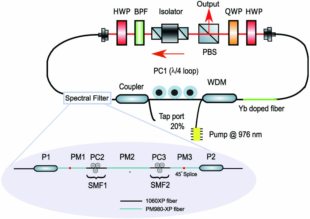
Fig. 1. Schematic of the fiber oscillator. PBS, polarizing beam splitter; HWP, half waveplate; QWP, quarter waveplate; BPF, bandpass filter; PC, polarization controller; WDM, wavelength division multiplexer; P, in-line polarizer; PM, polarization-maintaining; SMF, single mode fiber.

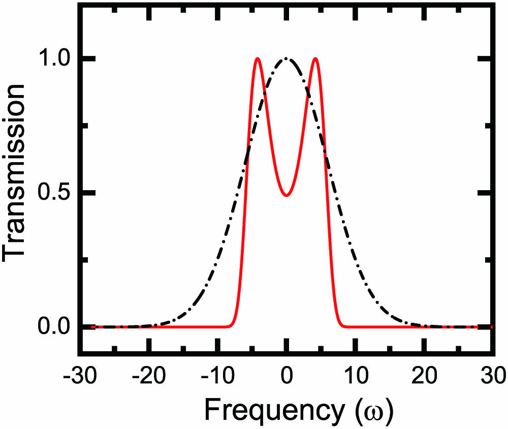
Fig. 2. Spectral filter transmission T(ω)=eδ−βω2−γω4 in the CQGLE model (dashed curve) with δ=0, β=0.012, and γ=0 and the CSHE model (solid curve) with δ=−0.7133, β=−0.0809, and γ=0.0023.

Fig. 3. Numerical simulation results. (a) Pulse evolution in the presence of the spectral filter. (b) Asymmetric pulse profile (blue curve) along with its chirp (red curve). (c) Amplitude contour plot explaining temporal dynamics of the moving pulse. (d) Asymmetric mode-locked spectrum (dashed blue curve) pertaining to the moving pulse solution in (c) and more asymmetric mode-locked spectrum (solid black curve) related to different simulation parameters. The inset shows the asymmetry at the longer wavelength tail of the spectra. (e) Pulse profile and the chirp associated with the more asymmetric mode-locked spectrum. (f) Temporal dynamics of the moving pulse solution related to the more asymmetric mode-locked spectrum.

Fig. 4. Output of the fiber-based filter and BPF combination (solid curve) with ASE (dashed line) as input. The dotted line depicts the output of fiber-based filter only.

Fig. 5. Experimental dataset recorded at 545 mW of input pump power. (a) Mode-locked spectrum at the PBS (solid curve) along with the spectral filter response (dashed curve). (b) Spectrum obtained at the 20% port of the fiber coupler. (c) Cross-correlation of the output pulse. (d) Pulse train. (e) RF spectrum. (f) Autocorrelation.

Fig. 6. Experimental dataset recorded at 571 mW of input pump power. (a) Mode-locked spectrum with a spectral filter response (dashed curve). (b) Cross-correlation of the output pulse. (c) Spectrum obtained at the 20% port of the fiber coupler. (d) Autocorrelation.

Fig. 7. Comparison between the two experimental datasets. (a) Asymmetry comparison between the two mode-locking states. The blue curve (spectrum 1) depicts the spectrum for the mode at 545 mW input pump power while the green curve (spectrum 2) denotes the spectrum for the mode measured at 571 mW. (b) Repetition rate comparison between the two spectra.