The ability of high-energy laser systems to provide complex laser pulse shapes has growing importance in many research disciplines such as laser fusion^[1–4], high-energy-density physics^[5–8], laboratory astrophysics^[9–11] and laser conditioning of optical materials^[12]. For example, X-ray diffraction of ramp-compressed crystalline solids can probe high-pressure phase transitions inaccessible with shock compression^[6]. In such laser facilities, accurate real-time predictions of laser performance are critical for maximizing experimental and operational effectiveness and flexibility. Several laser operation models that predict laser performance for high-energy laser systems have been reported^[13–22]. Most of these models utilize optimization methods that comprise forward propagation simulations with feedback to converge on the required on-target pulse power. This paper reports on PSOPS – a MATLAB^[23]-based semi-analytic model developed for the OMEGA EP^[24] laser system. PSOPS has been used to provide real-time accurate and rapid predictions of pulse shape, energy and near-field beam-fluence distribution in both forward and backward directions. In this article, we describe the PSOPS model, present examples of its prediction capability and show how its use has greatly enhanced the operational capabilities of OMEGA EP.

Essential features of PSOPS are (1) accurate, real-time predictions of expected performance of all four OMEGA EP beamlines within a small fraction of the OMEGA EP shot cycle; (2) an intuitive, easy-to-use interface for laser operators; (3) rapid optimization capability of the code between laser shots to fine-tune predictions based on shot performance; (4) forward and backward prediction capabilities. These features allow laser-system operators to quickly and accurately optimize laser pulse shape, energy and laser diagnostic filtrations prior to each OMEGA EP shot.

The paper is organized as follows. Section 2 describes the OMEGA EP laser-system architecture, emphasizing the key elements relevant to creating and characterizing complex ultraviolet (UV) pulse shapes. Section 3 discusses how PSOPS is used in shot operations, highlighting the need for a real-time semi-analytic model. Section 4 describes the model’s theoretical underpinnings, noting how the operational constraints within which OMEGA EP operates allow one to use an analytic solution to the coupled-rate and energy-transport equations that incorporates the measured beamline small-signal gain (SSG) with appropriate modifications to the Nd:glass saturation fluence. Section 5 compares PSOPS simulations with measurements; Section 6 describes facility enhancements that have been enabled by PSOPS. Finally, Section 7 presents a summary with a brief description of recent and planned upgrades to the model.

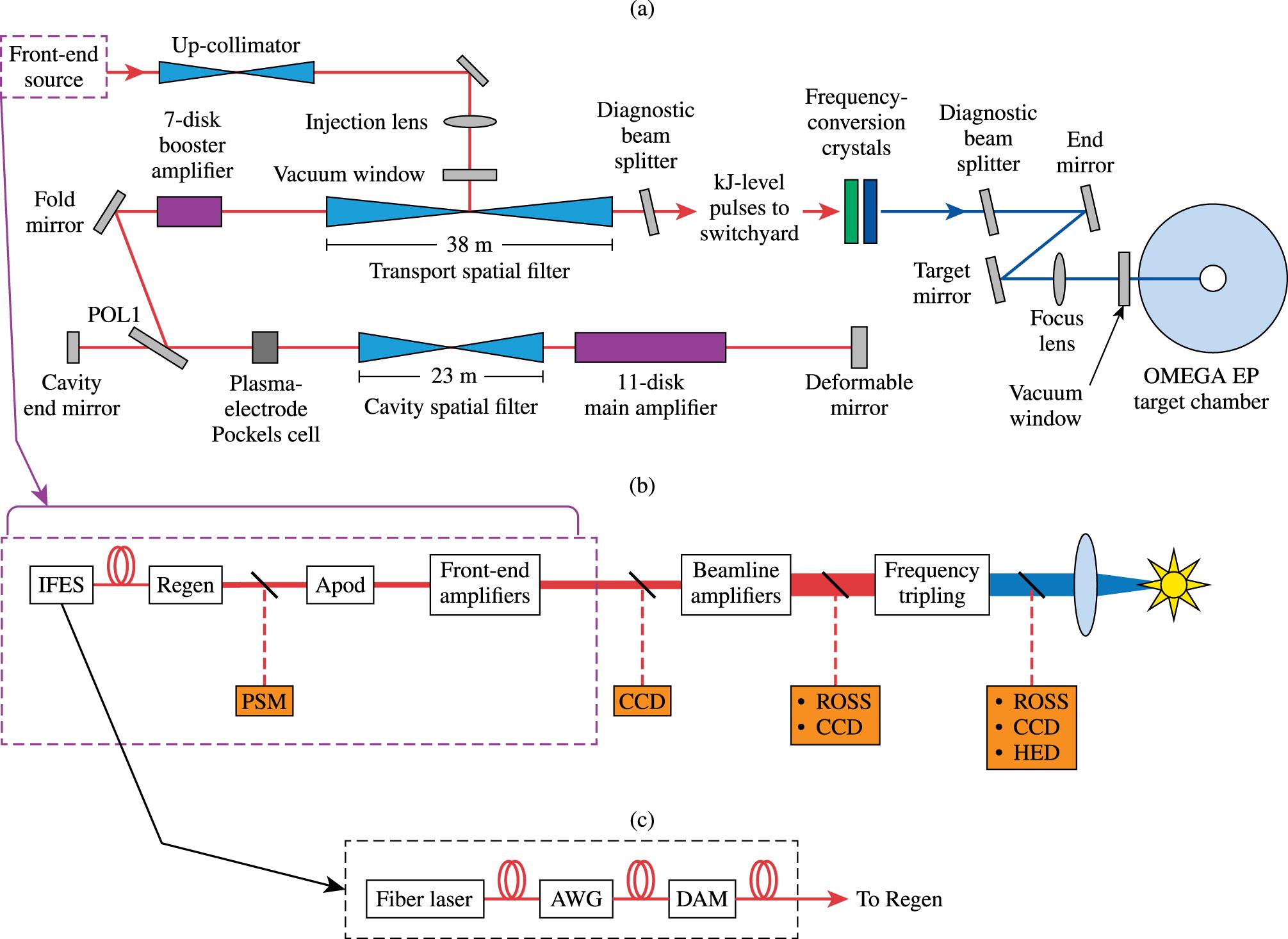
The OMEGA EP laser system is capable of producing either picosecond-scale infrared (IR) pulses (via optical parametric chirped-pulse amplification (OPCPA)) or nanosecond-scale UV pulses. For this paper, we confine our attention to the latter capability and will not consider the OPCPA operation further. Each of the four OMEGA EP beamlines uses a folded architecture based on the National Ignition Facility (NIF)^[25], as shown in Figure 1.

An integrated front-end system (IFES)^[26] produces temporally shaped 1053-nm seed pulses from a single-frequency, continuous-wave (cw) fiber laser. Precisely shaped temporal pulses are formed using an arbitrary waveform generator (AWG) that drives a dual-amplitude modulator. The resulting low-energy pulses, of between 0.1- and 10-ns duration, are injected into a diode-pumped regenerative amplifier (regen), which produces a cavity-dumped envelope of pulses from which a single pulse of ${\sim}5~\text{mJ}$ is switched out at the peak of the envelope^[27]. The pulse is then further amplified by flashlamp-pumped Nd:glass amplifiers^[28] prior to injection into the beamline. The laser pulse is then amplified by two passes through a 7-disk booster amplifier and four passes through an 11-disk main amplifier, both of which comprise 40-cm aperture, flashlamp-pumped Brewster angle and Nd-doped LHG-8 disks^{[29, 30]}. To support a wide range of shot energies and pulse durations, a variable number of the main-amplifier disks are actually pumped for a given shot. Compensation for the spatial gain variation produced by the beamline amplifier disks is provided by a beam-shaping apodizer in the front end^[31]. Frequency conversion to the third-harmonic wavelength is performed with a potassium dihydrogen phosphate (KDP) type-I doubler and a deuterated potassium dihydrogen phosphate (DKDP) type-II tripler^{[32, 33]}.

Laser pulse shape, energy and near-field beam profile are measured at several locations along the beam path. Diagnostic stages relevant to the PSOPS model and associated measurements are shown in Figure 1(b). The output pulse shape of each beamline’s regen is measured at a 5-Hz repetition rate using a photodiode-based pulse-stacking, pulse-shape monitor (PSM)^[34]. Calorimetrically calibrated charge-coupled-device (CCD) cameras (Scientific Instruments, model SI-800) are used to measure the near-field beam profile and laser-beam energy at the beamline injection and amplified beamline output stages. A harmonic energy diagnostic (HED)^[35] is used to measure the UV energy and the residual green and IR energy of the frequency-converted laser beam. Amplified IR and UV pulse shapes are measured using ROSS streak cameras^[36]. These diagnostic measurements are used to calibrate the PSOPS model and to determine the required stage energies and pulse shapes in both forward and backward directions when configuring for a shot, as described in Sections 3 and 4.

A major consideration in the development of the PSOPS model was to provide an accurate pulse-shape and energy prediction capability in both forward and backward directions that would give real-time guidance to the laser facility to satisfy the demands of rapidly evolving experimental campaign needs. This rapid prediction capability enables several performance enhancements for the facility that provide improved system performance accuracy and flexibility (see Section 6).

The PSOPS architecture allows one to run simulations in both the forward and backward directions, as illustrated in Figure 2. The model’s backward simulation capability is used to configure the system for a shot. In this case, the desired UV energy, pulse shape, expected beam profile and beamline amplifier configuration are provided as inputs to the PSOPS model. PSOPS produces the required pulse shape at the input of the system as well as the energies at each stage of the laser, from which the laser throttles and diagnostic configurations can be determined in a fast and robust manner.

During shot operations, PSOPS is used in the forward simulation direction to provide rapid predictions of laser-system performance using measured inputs to the amplifier chain. The measured input beam profile and real-time PSM-measured pulse shape are used with the expected beamline injected energy and previously measured beamline SSG to predict the IR and frequency-converted UV performance at the end of the beamline. Pulse-shape distortion through the remainder of the front end after the regen is minimal because front-end Nd:glass laser amplifiers are maintained sufficiently below gain-saturation conditions. A front-end qualification shot is taken at the start of a shot day to confirm the expected injected energy and to measure the injected beam’s near-field distribution that is used as input to the PSOPS model. A graphical user interface (GUI) that displays the predicted and requested UV power allows laser operators to adjust pulse shapes and verify expected on-target UV energy between shots. The predicted stage energies are also displayed on the GUI and compared to the expected values.

In high-pulse-energy laser systems, efficient energy extraction from the laser gain medium requires that the laser fluence should approach the medium’s saturation fluence. Such laser operation depletes the inversion leading to temporally dependent saturation of the gain, which, in a pulsed laser system, causes the output pulse to become temporally distorted. Analytic solutions to the coupled-rate and energy-transport equations for a homogeneously saturating thin slab are used in PSOPS to determine the time-dependent gain within each laser disk at discrete locations across the laser aperture. The four-level equations can be expressed as^[37]$$\begin{eqnarray}\displaystyle & & \displaystyle \frac{\unicode[STIX]{x1D6FF}n_{3}}{\unicode[STIX]{x1D6FF}t}=W_{p}n_{0}+c\unicode[STIX]{x1D719}\unicode[STIX]{x1D70E}_{23}n_{2}-\frac{n_{3}}{\unicode[STIX]{x1D70F}_{32}},\end{eqnarray}$$ (1)$$\begin{eqnarray}\displaystyle & & \displaystyle \frac{\unicode[STIX]{x1D6FF}n_{2}}{\unicode[STIX]{x1D6FF}t}=c\unicode[STIX]{x1D719}\unicode[STIX]{x1D70E}_{12}n_{1}-c\unicode[STIX]{x1D719}(\unicode[STIX]{x1D70E}_{21}+\unicode[STIX]{x1D70E}_{23})n_{2}-\frac{n_{2}}{\unicode[STIX]{x1D70F}_{21}}+\frac{n_{3}}{\unicode[STIX]{x1D70F}_{32}},\qquad\end{eqnarray}$$ (2)$$\begin{eqnarray}\displaystyle & & \displaystyle \frac{\unicode[STIX]{x1D6FF}n_{1}}{\unicode[STIX]{x1D6FF}t}=c\unicode[STIX]{x1D719}\unicode[STIX]{x1D70E}_{21}n_{2}-c\unicode[STIX]{x1D719}\unicode[STIX]{x1D70E}_{12}n_{1}+\frac{n_{2}}{\unicode[STIX]{x1D70F}_{21}}-\frac{n_{1}}{\unicode[STIX]{x1D70F}_{10}},\end{eqnarray}$$ (3)$$\begin{eqnarray}\displaystyle & & \displaystyle \frac{\unicode[STIX]{x1D6FF}n_{0}}{\unicode[STIX]{x1D6FF}t}=-W_{p}n_{0}+\frac{n_{1}}{\unicode[STIX]{x1D70F}_{10}},\end{eqnarray}$$ (4)$$\begin{eqnarray}\displaystyle & & \displaystyle \frac{\unicode[STIX]{x1D6FF}\unicode[STIX]{x1D719}}{\unicode[STIX]{x1D6FF}t}+c\frac{\unicode[STIX]{x1D6FF}\unicode[STIX]{x1D719}}{\unicode[STIX]{x1D6FF}z}=c\unicode[STIX]{x1D719}(\unicode[STIX]{x1D70E}_{21}n_{2}-\unicode[STIX]{x1D70E}_{12}n_{1}-\unicode[STIX]{x1D70E}_{23}n_{2}),\end{eqnarray}$$ (5) where $n_{i}(n=0,1,2,3)$ are the population densities of the levels, $c$ is the speed of light in the medium, $\unicode[STIX]{x1D719}$ is the photon number density, $W_{p}$ is the pumping rate, $\unicode[STIX]{x1D70E}_{23}$ is the effective excited-state absorption cross section out of the upper laser level, $\unicode[STIX]{x1D70E}_{12}$ and $\unicode[STIX]{x1D70E}_{21}$ are the effective stimulated absorption and emission cross sections, respectively, and $\unicode[STIX]{x1D70F}_{32}$, $\unicode[STIX]{x1D70F}_{21}$ and $\unicode[STIX]{x1D70F}_{10}$ are the decay times of the pump level, laser transition and terminal laser level, respectively. We assume that the transition from the pump band into the upper laser level occurs very rapidly and that the lifetime of the upper laser level is long compared to the laser pulse’s transit time^[38]. We also assume that temporal variations in the inversion produced by the pump are small during the stimulated emission process that amplifies the laser pulse^[39]. The main discharge current pulse to the amplifier flashlamps has a width of greater than $300~\unicode[STIX]{x03BC}\text{s}$, and its peak is timed to coincide with the arrival of the laser pulse in the amplifier, whereas the maximum laser pulse width on OMEGA EP is currently 10 ns and a round-trip time through the beamline amplifier disks is approximately 700 ns. We assume that there is negligible excited-state absorption or other up-conversion losses ($\unicode[STIX]{x1D70E}_{23}\sim 0$) since the available inversion and the gain profile in the OMEGA EP disks are dominated by amplified spontaneous emission (ASE) depumping^[40], which is taken into account in the PSOPS model by using the measured SSG. As will be shown, the use of the measured beamline SSG in the model and the ability to optimize the model’s fitting parameters between SSG measurements effectively take into account inversion losses that limit the available gain. The terminal-level decay time $\unicode[STIX]{x1D70F}_{10}$ is only a significant contributor to the amplification process for pulse widths $\unicode[STIX]{x1D70F}\sim \unicode[STIX]{x1D70F}_{10}$ and does not contribute significantly to most OMEGA EP pulse shapes, but it will be taken into account by using an empirically derived modification to the saturation fluence^[41]. We therefore assume for now that the terminal-level lifetime is much shorter than the pulse width of the laser such that $n_{1}\sim 0$. It will be shown that a further modification to the saturation fluence also takes into account glass host matrix contributions to inhomogeneous broadening^[42]. With these simplifying assumptions, the relevant equations in the frame of the laser pulse are $$\begin{eqnarray}\displaystyle \frac{\unicode[STIX]{x1D6FF}n_{2}(z,t)}{\unicode[STIX]{x1D6FF}t} & = & \displaystyle -\frac{I(z,t)}{\hslash \unicode[STIX]{x1D714}}\unicode[STIX]{x1D70E}_{21}n_{2}(z,t),\end{eqnarray}$$ (6)$$\begin{eqnarray}\displaystyle \frac{\unicode[STIX]{x1D6FF}I(z,t)}{\unicode[STIX]{x1D6FF}z} & = & \displaystyle I(z,t)\unicode[STIX]{x1D70E}_{21}n_{2}(z,t),\end{eqnarray}$$ (7) where $I(z,t)=c\unicode[STIX]{x1D719}(z,t)\hslash \unicode[STIX]{x1D714}$ is the laser pulse intensity at photon frequency $\unicode[STIX]{x1D714}$, $\hslash$ is Planck’s constant, and the dependence on propagation distance and time is explicitly shown. These coupled equations in ($z,t$) can be reduced to coupled equations in $t$ only and solved to obtain the time-varying partially saturated gain in the time frame of the laser pulse. This partially saturated gain can be expressed in terms of the input or output pulses of the laser amplifier and the initial gain prior to arrival of the pulse as^{[43, 44]}$$\begin{eqnarray}G_{\text{in}}(t)=\frac{1}{1-(1-G_{0}^{-1})\exp [-F_{\text{in}}(t)/F_{\text{sat}}]}\end{eqnarray}$$ (8) or $$\begin{eqnarray}G_{\text{out}}(t)=1+(G_{0}-1)\exp [-F_{\text{out}}(t)/F_{\text{sat}}],\end{eqnarray}$$ (9) where $G_{0}$ is the initial gain, $F_{\text{sat}}$ is the saturation fluence, $$\begin{eqnarray}F_{\text{sat}}=\frac{\hslash \unicode[STIX]{x1D714}}{\unicode[STIX]{x1D70E}_{21}},\end{eqnarray}$$ (10) and $$\begin{eqnarray}\displaystyle F_{\text{in}}(t)\equiv \displaystyle \int _{t_{0}}^{t}I_{\text{in}}(t^{\prime })\,\text{d}t^{\prime }, & & \displaystyle\end{eqnarray}$$ (11)$$\begin{eqnarray}\displaystyle F_{\text{out}}(t)\equiv \displaystyle \int _{t_{0}}^{t}I_{\text{out}}(t^{\prime })\,\text{d}t^{\prime }. & & \displaystyle\end{eqnarray}$$ (12)

The integrals in Equations (11) and (12) are taken from the starting time $t_{0}$ of the pulse up to the normalized time $t$ within the pulse. The output pulse can be determined from a given input pulse using Equation (8) as $$\begin{eqnarray}I_{\text{out}}(t)=G_{\text{in}}(t)I_{\text{in}}(t),\end{eqnarray}$$ (13) whereas Equation (9) can be used to determine the input pulse required to produce a desired output pulse, $$\begin{eqnarray}I_{\text{in}}(t)=I_{\text{out}}(t)/G_{\text{out}}(t).\end{eqnarray}$$ (14) Note that the inversion dependence in $z$ need not be considered and that for each time $t$ in the pulse, the gain is dependent only on the initial gain $G_{0}$ and the accumulated energy per unit area from time $t_{0}$ compared to the saturation fluence. The gain dependence in $z$ could, in principle, be calculated, which may be important for subsequent passes in cases where the terminal-level lifetime is long^[45–47]; however, as will be shown, the use of the initial gain $G_{0}$ for each of the multiple passes through a laser disk is a valid approximation for the OMEGA EP beamline. We note that a similar semi-analytic approach to determine input and output pulse shapes has been used in a quasi-three-level, all-fiber amplifier chain^[48].

In the absence of losses or higher-order effects contributing to pulse-shape distortion, Equations (8)–(14) imply that a precise knowledge of the initial gain $G_{0}$ and saturation fluence $F_{\text{sat}}$ is sufficient to determine the input or output pulse shapes. In the PSOPS model, the time-dependent gain is determined at discrete locations across the laser aperture, where the initial gain $G_{0}(x,y)$ is taken as the measured SSG of each disk, and the saturation fluence is inferred from prior beamline input versus output energy measurements under gain-saturation conditions. For multi-pass amplification, each laser amplifier disk is treated as a thin slab and either Equation (13) or (14) is applied iteratively per disk for forward or backward prediction, respectively^[45]. Therefore, for forward prediction, the output intensity of disk $k$ is given by $$\begin{eqnarray}I_{k}(t,x,y)=\unicode[STIX]{x1D6FD}^{2}\cdot G_{k}(t,x,y)I_{k-1}(t,x,y),\end{eqnarray}$$ (15) where $$\begin{eqnarray}\displaystyle & & \displaystyle \hspace{-18.0pt}G_{k}(t,x,y)\nonumber\\ \displaystyle & & \displaystyle \hspace{-12.0pt}\quad =\frac{1}{1-\{1-[G_{0}(x,y)]^{-1}\}\exp [-F_{k}(t,x,y)/F_{\text{sat}}]},\end{eqnarray}$$ (16)$$\begin{eqnarray}\displaystyle & & \displaystyle \hspace{-18.0pt}F_{k}(t,x,y)=\displaystyle \int _{t_{0}}^{t}\unicode[STIX]{x1D6FD}\cdot I_{k-1}(t^{\prime },x,y)\,\text{d}t^{\prime },\end{eqnarray}$$ (17) and a per-disk-surface loss factor $\unicode[STIX]{x1D6FD}$ is included in the model to account for passive losses. The SSG and saturation fluence at any location ($x$, $y$) within the beam are both taken as constant for the propagation distance through a single disk. Following the repeated application of Equations (15)–(17) through the entire beamline, frequency conversion to the third harmonic uses look-up tables from MIXER calculations^{[32, 33]}. For backward prediction starting with the UV-beam profile, pulse shape and energy, these tables provide the amplified IR intensity at the end of the beamline from which the beamline input intensity is recursively calculated using the following equations: $$\begin{eqnarray}\displaystyle I_{k}(t,x,y) & = & \displaystyle I_{k+1}(t,x,y)/\unicode[STIX]{x1D6FD}^{2}\cdot G_{k}(t,x,y),\end{eqnarray}$$ (18)$$\begin{eqnarray}\displaystyle G_{k}(t,x,y) & = & \displaystyle 1+[G_{0}(x,y)-1]\exp [-F_{k}(t,x,y)/F_{\text{sat}}],\nonumber\\ \displaystyle & & \displaystyle\end{eqnarray}$$ (19)$$\begin{eqnarray}\displaystyle F_{k}(t,x,y) & = & \displaystyle \displaystyle \int _{t_{0}}^{t}[I_{k+1}(t^{\prime },x,y)/\unicode[STIX]{x1D6FD}]\text{d}t^{\prime },\end{eqnarray}$$ (20) where $I_{k}$ ($t,x,y$) is the input intensity of the $k$th disk.

The saturation fluence for Nd:glass laser media given by Equation (10) must be modified to account for an inhomogeneous broadening effect in the laser glass^[42] and for bottlenecking of the terminal level of the lasing transition for pulse widths close to the terminal-level lifetime $\unicode[STIX]{x1D70F}_{10}$, where $\unicode[STIX]{x1D70F}_{10}\sim 0.25$ ns for Nd-doped phosphate laser glasses^{[41, 49]}. The effective saturation fluence of the OMEGA EP beamline is dependent on the beamline’s output fluence and has been inferred from prior fits to gain-saturation data, as shown in Figure 3. The optimization fits from which the plot in Figure 3 was derived were done to the measured UV power using PSOPS forward predictions while adjusting the loss term $\unicode[STIX]{x1D6FD}$ and effective cross-section term $\unicode[STIX]{x1D70E}_{21}$ in the model, and the fit values have been scaled to account for Brewster angle incidence on the disks in order to compare with literature values. To reduce the effect of pulse width on the determination of saturation fluence, shot data included only pulse widths of 2 ns or greater; to reduce the contribution of measurement error and pulse-shape temporal modulation, only beam output energies of greater than ${\sim}2~\text{kJ}$ were used, where the pulse-shape distortion from gain saturation was large^[50]. The measured effect is consistent with that reported for LHG-8^[51] and for LG-750^[42], where the composition is similar to that of the LHG-8 laser glass used in OMEGA EP^[52]. The inferred saturation fluence for any given output fluence in Figure 3 must be interpreted as an average over all amplifier disks, where significant saturation occurs through only the last pass of the cavity and booster amplifiers. Nonetheless, in Section 5, we show that the use of this saturation fluence as a fitting parameter for the model has provided robust agreement between model simulations and measurements.

Assuming negligible pumping during the laser pulse width $\unicode[STIX]{x1D70F}$, an additional modification to the saturation fluence is used to account for bottlenecking of the terminal laser level^[41]: $$\begin{eqnarray}F_{\text{sat}}^{\prime }=\frac{\hslash \unicode[STIX]{x1D714}/\unicode[STIX]{x1D70E}_{\text{em}}}{\unicode[STIX]{x1D6FE}(R)},\end{eqnarray}$$ (21) where $$\begin{eqnarray}\unicode[STIX]{x1D6FE}(R)=1+K\cdot B(R)\end{eqnarray}$$ (22) and $\unicode[STIX]{x1D70E}_{\text{em}}$ is the effective emission cross section determined from the optimization fits; $\unicode[STIX]{x1D6FE}(R)$ is an empirical scaling factor whose value is dependent on the ratio $R=\unicode[STIX]{x1D70F}/\unicode[STIX]{x1D70F}_{10}$; $K=0.35$ is an effective degeneracy ratio for the upper and lower Nd manifolds in Nd-doped phosphate glass; the empirical function $B(R)$ was determined in Ref. [41]. The dependence of $[\unicode[STIX]{x1D6FE}(R)]^{-1}$ on laser pulse width $\unicode[STIX]{x1D70F}$ is plotted in Figure 4. This correction to the saturation fluence generally has a small effect on the predicted beam output energy for most OMEGA EP pulses. For a 1-ns square pulse, the modified saturation fluence can provide an improvement in predicted beam output energy of the order of 1% but this is generally less than the error between simulated and measured energies on the first shot of the day (see Section 6.1). Greater improvement would be expected for shorter pulses, but an accurate assessment is currently limited by the impulse response of the regen pulse measurement (see Section 5).

For subsequent passes of the laser pulse through an amplifier disk, some amount of gain recovery might be expected, owing to drain of the terminal level. In this case, the terminal-level population would be reduced to $\exp (-T/\unicode[STIX]{x1D70F}_{10})$ of its value immediately after passage of the pulse, where T is the round-trip time between passes^{[45, 53]}. In the OMEGA EP beamline, the shortest round-trip time, and therefore the least amount of gain recovery, would be expected for the main cavity disk closest to the beamline deformable mirror (DM, Figure 1), where the round-trip time between the disk and the DM is 22 ns. In this case, $\exp (-22~\text{ns}/0.25~\text{ns})\sim 10^{-38}$, thereby justifying the assumption of full gain recovery between passes and the use of the same initial gain distribution for each pass of a beamline disk. The beamline SSG measured with a 10-ns square pulse is used in the PSOPS model, as described in Section 4.4. Using the measured SSG effectively takes into account inversion losses such as from ASE depumping, flashlamp or reflector degradation and gain recovery for subsequent passes through the amplifier resulting from terminal-level drain.

The spatially dependent, single-pass SSG for each amplifier disk used in the model is derived from full-system SSG measurements for the seven-disk booster-amplifier configuration and for each main-amplifier configuration to be used during shot operations. The SSG is measured by dividing calorimetrically calibrated beam-fluence measurements at the injection plane and beamline output. The resulting beam ratio for an amplified shot in the small-signal regime is divided by the same ratio with the amplifier disks unpumped, thereby eliminating the contribution from passive loss. The single-disk SSG $G_{0}(x,y)$ is taken as the geometric mean for each measurement, $$\begin{eqnarray}G_{0}(x,y)=\left\{\frac{[F_{\text{out}}(x,y)/F_{\text{in}}(x,y)]_{\text{pumped}}}{[F_{\text{out}}(x,y)/F_{\text{in}}(x,y)]_{\text{unpumped}}}\right\}^{1/N},\end{eqnarray}$$ (23) where $F_{\text{in}}(x,y)$ and $F_{\text{out}}(x,y)$ are the temporally integrated, measured beamline input and output fluence profiles, respectively, and $N=d\cdot p$, where $d$ is the number of disks configured and $p$ is the number of passes through the disk. A separate SSG measurement is made for the main cavity- and booster-amplifier sections of the beamline. The single-disk SSG is taken as the geometric mean for each measurement. For example, Figure 5 shows a 15th-order Legendre fit to the measured nine-disk, four-pass cavity total SSG (Figure 5(a)) and the inferred single-disk SSG (Figure 5(b)). Figure 6 shows column-averaged, horizontal lineouts through the single-disk SSG distributions for different numbers of main-amplifier disks fired. The cavity disk at the end of the amplifier chain is pumped only in the odd-disk configuration and the asymmetric distribution of flashlamp light across the end disk results in the asymmetric gain profile seen in Figure 6(a)^[29].

The optimization from which Figure 3 was derived was performed to the measured UV power while adjusting the loss and effective cross-section terms as fitting parameters. The frequency-conversion model has been previously calibrated to achieve excellent agreement between simulated and measured third-harmonic conversion efficiency. For the IR beamline section of the model, two different forms of the model have been used and have achieved similar accuracy.

The first method is an extension of the optimization done in Figure 3. When the model begins to show a loss of accuracy, a single optimization fit is performed if a recent high-energy shot is available. A check is done to ensure that the $\unicode[STIX]{x1D70E}_{\text{em}}$ fit value is within the previously determined range of inferred values. This calibration can be done within a few minutes between OMEGA EP shots. Once the model is calibrated, subsequent forward predictions use a quasi-Newton method to determine the correct saturation fluence where a low-resolution spatial grid is propagated in the forward direction using an initial value of saturation fluence. The average fluence of the output beam is then used to adjust the saturation fluence per the slope in Figure 3 iteratively until a convergent value of saturation fluence is determined. This final value of the saturation fluence is then scaled for pulse-width dependence and used for the final forward simulation, which may be of higher spatial resolution. The quasi-Newton method used for forward predictions is illustrated by the flowchart in Figure 7. For backward simulation starting with a UV beam and pulse, the backward-simulated IR beamline output fluence is used directly to calculate the required saturation fluence per the most recent $\hslash \unicode[STIX]{x1D714}/\unicode[STIX]{x1D70E}_{\text{em}}$ fit value and slope from Figure 3.

In the second method, the local saturation fluence for each grid point and amplifier disk is determined per the equation in Figure 3 for both forward and backward simulations. For the forward simulation, Equation (16) takes the form, $$\begin{eqnarray}\displaystyle & & \displaystyle G_{k}(t,x,y)\nonumber\\ \displaystyle & & \displaystyle =\frac{1}{1-\{1-[\unicode[STIX]{x1D6FC}\cdot G_{0}(x,y)]^{-1}\}\exp [-F_{k}(t,x,y)/F_{\text{sat},k}(x,y)]},\nonumber\\ \displaystyle & & \displaystyle\end{eqnarray}$$ (24) where $$\begin{eqnarray}F_{\text{sat},k}(x,y)=\frac{m\displaystyle \int _{-\infty }^{\infty }\unicode[STIX]{x1D6FD}\cdot I_{k-1}(t,x,y)\,\text{d}t+b}{\unicode[STIX]{x1D6FE}(R)},\end{eqnarray}$$ (25) and $m=0.082$ and $b=3.741$ are the fit values shown in the plot of Figure 3; $\unicode[STIX]{x1D6FC}$ is a multiplier on the SSG; the correction for the finite lifetime of the terminal laser level is explicitly shown. Optimization to the measured UV power is performed in the forward direction using the per-disk-surface loss term $\unicode[STIX]{x1D6FD}$ and the factor $\unicode[STIX]{x1D6FC}$ as fit variables. For the backward simulation, Equation (19) becomes $$\begin{eqnarray}\displaystyle G_{k}(t,x,y) & = & \displaystyle 1+[\unicode[STIX]{x1D6FC}\cdot G_{0}(x,y)-1]\nonumber\\ \displaystyle & & \displaystyle \times \,\exp [-F_{k}(t,x,y)/F_{\text{sat},\text{k}}(x,y)],\end{eqnarray}$$ (26) where $$\begin{eqnarray}F_{\text{sat},k}(x,y)=\frac{m\displaystyle \int _{-\infty }^{\infty }[I_{k+1}(t,x,y)/\unicode[STIX]{x1D6FD}]\text{d}t+b}{\unicode[STIX]{x1D6FE}(R)}.\end{eqnarray}$$ (27) In practice, we have found similar accuracy with both methods, although the first method (quasi-Newton) has generally been more robust for a broad range of energies and pulse shapes. The results shown in the following sections have therefore used this method. The simulation and calibration sequence can thus be summarized as follows.(1)

Backward simulation using requested UV pulse shape, energy, and beam profile to calculate required regen pulse shape, stage energies, system throttles, and laser diagnostic filtrations.

Spatial and temporal simulations in both forward and backward directions are in excellent agreement with measurements, as shown in Figures 8 and 9, respectively. The shot data shown in these figures were obtained using the configuration of nine main amplifiers and seven booster amplifiers, and the model was calibrated using an earlier shot where beamline gain saturation was large.

Since the calibrated loss term $\unicode[STIX]{x1D6FD}$ and the inferred saturation fluence data in the plot of Figure 3 are an average over all amplifier disks using the configuration (mentioned above) of nine main amplifiers and seven booster amplifiers, there is some question concerning the accuracy of the simulations when different amplifier configurations are used. To test the accuracy of the model when the number of main amplifiers is different than that used for model calibration, PSOPS simulations were performed on shots used for SSG measurements. The model was first calibrated to a high-fluence UV shot using SSG maps for the nine-main-amplifier and seven-booster-amplifier configurations, and this calibration was used to simulate the beamline IR output energies for SSG shots using fewer than nine main amplifiers and no booster amplifiers, where the measured single-disk SSG map for each unique main-amplifier configuration was used in the simulations. The agreement between simulated and measured beamline output IR energies is excellent, as shown in Table 1.

These results highlight the following important considerations. First, the measured single-disk SSG map for each unique main-amplifier configuration must be used to achieve good agreement with measurements (see Figure 6). Second, the use of a single loss parameter $\unicode[STIX]{x1D6FD}$ and the inferred saturation fluence as fitting parameters, determined using the method of Section 4.5, provides good agreement with measurements over a wide range of amplifier configurations and beam output fluences. Although beamline output fluences for the cases shown in Table 1 were in the small-signal regime, the calibration shot was taken in a regime where square-pulse distortion and beamline saturation were large. The accuracy of the model over a large range of fluences and saturation levels is further illustrated in Section 6. Third, if changes in SSG differ over time for each configuration, the model’s ability to accurately predict stage energies for different amplifier configurations may not be as robust as shown in Table 1. In this case, the first shot of the day may be used to make small adjustments to calibration factors $\unicode[STIX]{x1D6FC}$ or $\unicode[STIX]{x1D6FD}$, or a new optimization of the model’s fitting parameters may be performed using the desired beamline configuration. New SSG measurements may also be taken if significant changes in SSG profile are suspected.

For 100-ps pulses, we found that forward simulations were in good agreement with beamline output IR energy measurements, but simulated UV energy and pulse width were too low and too wide, respectively (Figure 10(a)). Backward simulations, however, showed excellent agreement with measured beamline injected energies, while the simulated injected pulse width was shorter than the measured injected pulse width. These discrepancies suggested that the impulse response of the input pulse measurement system was insufficient for accurate prediction of peak frequency-conversion efficiency. For more accurate forward predictions, the impulse response of the pulse-shape measurement system has been estimated using the measured UV pulse shape, energy and PSOPS backward simulation. A forward simulation for a different shot using the deconvolved measurement of its input pulse shape produced much better agreement with the measured UV pulse power and stage energies (Figure 10(b)). Based on these results, we are currently characterizing the impulse response of the injected pulse measurement system to determine what improvements need to be made.

The unique features of PSOPS have provided greater performance accuracy and flexibility by enabling rapid optimization in key areas.Determination of front-end throttle and pulse-shape adjustments required to compensate for such issues as changes in passive loss through a beamline, loss of gain from amplifier flashlamp degradation, spatial variations in saturated gain resulting from changes in injected beam profile and spatiotemporal variations in regen performance. This has improved OMEGA EP’s ability to accurately produce users’ requested UV energies and pulse shapes.Adjustments to on-target energy and pulse shape within predetermined allowances based on a user’s real-time analysis of experimental data.Increased effective pulse-duration range through precise concatenation of pulses across multiple beams.Improved system alignment. As a post-shot analysis and diagnostic tool, PSOPS has been used to guide alignment of beam-shaping apodizers in the front end of OMEGA EP and to understand the effects of beamline-centering errors in order to optimize the fill factor of the amplified beam, reduce near-field modulation and help elucidate causes of beamline gain changes.

These improvements are described in detail below.

Drifts in system performance can lead to noticeable deviations between simulated and achieved pulse shapes and energies, which can be minimized with an agile system model such as PSOPS. For example, Figure 11 shows how optimization of the injected pulse shape can be done for small changes in system performance. Although the nominal AWG pulse shape is determined prior to shot day, small changes in regen performance on shot day can significantly affect the UV pulse shape. For example, the left plot in Figure 11(a) shows a prediction of the expected UV pulse based on the pre-shot PSM measurement of the regen pulse that departs from the ideal pulse shape near the end of the pulse. Based on this prediction, the AWG waveform was modified to provide the compensated pre-shot prediction shown on the right in Figure 11(a). The post-shot UV simulation showed excellent agreement with the measurement (Figure 11(b)).

Although the AWG adjustment is not currently a closed loop, the regen performance is typically sufficiently stable so that only minor adjustments are required. Closed-loop AWG waveform optimization will be implemented in the near future. In addition to changes in regen performance, small changes in beamline gain and losses may result in approximately 5% discrepancy between the measured and simulated UV energy on the first shot of the day, in which case the model can be calibrated before the second shot based on the measured pulse power, as described in Section 4. The optimized simulated UV energy is typically within ${\sim}1\%$ of the measurement on the second shot of the day.

PSOPS has also enhanced laser facility flexibility by enabling users to adjust requested UV pulse shapes and energies between laser shots within a predefined range that is determined uniquely for each experimental campaign. The allowed range of energy and pulse-shape modification is assessed with respect to the laser system’s fluence limits, the range of energy and pulse shapes planned for the day and the likelihood of maintaining each beamline’s 90-minute shot cycle. In the example shown in Figure 12(a), a significant increase in the slope of the UV pulse was desired following a laser shot while maintaining 220 J of UV on-target energy. In Figure 12(b), different energies were desired while maintaining the original normalized design pulse shape that produced 500 J of UV on-target energy. These requests were based on each user’s real-time analysis of experimental data and were accommodated in each case by adjusting the front-end pulse shape and throttles per the PSOPS pre-shot prediction.

Most of the discrepancies between the requested and measured pulse shapes in Figure 12 can be understood by noting that the corresponding IR beam intensities entering the frequency-conversion crystals were close to the small-signal regime for frequency tripling, where the third-harmonic intensity is proportional to the third power of the IR intensity^[33]. Thus, small uncorrected deviations from the ideal regen pulse shapes produced significantly larger deviations in the frequency-converted pulse shapes. We expect that the automated adjustment of the AWG waveform will allow improved pulse-shape optimization to be performed within OMEGA EP’s 90-minute shot-cycle time.

Currently, OMEGA EP’s regens can accommodate single beamline pulse widths of up to 10 ns. However, improved system modeling in conjunction with precision timing allows the technique of pulse stitching to achieve up to a $4\times$ increase in effective pulse duration. With pulse stitching, as illustrated in Figure 13, pulse shapes from different beamlines can be precisely combined on target to form a single composite pulse shape. The composite 27-ns ramped pulse shape shown in Figure 13 was formed by incoherent addition of the individual pulses, separated by the temporal delay between them. Prior to the shot, PSOPS is used to predict the composite pulse, given the specified beam-to-beam temporal delay (Figure 13(a)). The measured composite pulse shown in Figure 13(b) was formed using the individual beamline pulse-shape measurements and the measured beam-to-beam UV pulse timing.

We note that all four long-pulse beams are derived from the same single-frequency oscillator, and the focusing optic assemblies on the OMEGA EP target chamber are mounted such that the beams form a cone of approximately $23^{\circ }$ half-angle with the vertex of the cone at target chamber center. Therefore, the incoherent sum used to form the composite pulse does not take into account high-frequency modulation that may occur on target in the pulse overlap regions.

PSOPS has been used as a tool to optimize the alignment of beam-shaping apodizers in the Sources front end (see Figure 1). PSOPS predictions of the effect of small changes in beam centering and rotation on the amplified near-field beam uniformity can be used as a guide to optimize the apodizer alignment without requiring amplified shots. This has resulted in a better understanding of required tolerances for centering and rotating both the beam-shaping apodizer and the apodized injected beam with respect to the gain profile of the beamline. As an example, Figure 14 shows the measured effect that identifying and correcting a small error in apodizer alignment has on the amplified IR near-field beam. Using the measured injected near-field beam, PSOPS forward simulations were used to predict the amplified beamline output near-field profile and to correct the apodizer’s alignment with respect to the gain profile of the beamline within a 10-minute shot cycle. A 0.49-mm shift of the apodizer improved the output beam quality, both in terms of the fluence contrast (from 13.1% to 9.4%) and the peak-to-mean fluence ratio (from 1.46:1 to 1.43:1). Fluence contrast is defined as the standard deviation of the fluence divided by the mean fluence value.

PSOPS has also been used to perform iterative, multi-axis optimization of the apodizer alignment to reduce the peak fluence of the frequency-converted UV beam. Figure 15 shows that a rotation of the apodizer by $3.5^{\circ }$, followed by lateral shifts of 0.36 mm (horizontal) and 0.24 mm (vertical) reduced the peak-to-mean UV-beam fluence from 3.74:1 (Figure 15(a)) to 2.76:1 (Figure 15(d)) using the same beamline saturation conditions. The improved near-field profile shown in Figure 15(d) was achieved using iterative PSOPS predictions followed by a single amplified UV shot. By limiting near-field beam fluence, fluence-limited damage may be avoided, leading to enhanced energy performance. The quality of the regen beam that was incident on the apodizer contributed to the residual nonuniformity seen in Figure 15(d), suggesting that further reduction in UV-beam peak fluence may be possible by improving the regen-output beam quality, for which the model can also be used as a guide owing to its accurate and rapid prediction capability. For example, PSOPS has been used during front-end qualification as a post-shot analysis tool to assess whether residual nonuniformity of the front-end near-field beam is acceptable for the given shot campaign, or whether additional laser facility time should be used to improve the beam uniformity. These measurements, guided by PSOPS simulations, have provided a better understanding of laser-system contributions to the amplified UV-beam profile and, importantly, have demonstrated that small adjustments to apodizer alignment are often sufficient to correct near-field beam nonuniformity in lieu of designing and manufacturing new apodizers.

PSOPS is a semi-analytic model that is used on the UV beamlines of OMEGA EP to rapidly predict pulse shapes, stage energies and near-field beam distributions in both forward and backward directions and has enabled several enhancements to laser-system performance accuracy and flexibility. The use of analytic solutions to the coupled-rate and energy-transport equations, with incorporation of the measured SSG and appropriate modifications to the saturation fluence, has enabled accurate and rapid optimization of laser-system performance within a small fraction of the OMEGA EP 90-minute shot cycle. PSOPS is the key enabler of an automated capability to compute and specify the laser system’s stage energies and corresponding diagnostic filtrations prior to each OMEGA EP shot based on evolving on-target pulse-shape and energy requirements. In conjunction with precision timing, the model has allowed the technique of pulse stitching to achieve up to a 4$\times$ increase in effective pulse duration. The backward simulation capability allows for rapid convergence of the predicted and requested on-target UV pulse power. The ability to calibrate the model between laser shots accounts for day-to-day system drifts without loss of shot time. The model has also been used to clarify the cause of laser-beam profile changes and the acceptable tolerance for beam alignment. Adjustments to beam-shaping apodizer alignment predicted by PSOPS have been used to improve the amplified near-field beam uniformity in lieu of designing and manufacturing new apodizers. A referential database archives laser and model performance and model versions. An upgrade to the model currently in progress accounts for the spectral dependence of beamline gain for shots that require spectrally tunable UV on-target irradiation to mitigate cross-beam energy transfer^[54]. This will be refined to account for spectral dependence of effective cross section and saturation fluence. In addition, we anticipate that closed-loop AWG adjustments will further reduce the time required for pulse-shape design and setup.

References

[1] S. X. Hu, W. Theobald, P. B. Radha, J. L. Peebles, S. P. Regan, A. Nikroo, M. J. Bonino, D. R. Harding, V. N. Goncharov, N. Petta, T. C. Sangster, E. M. Campbell. Phys. Plasmas, 25(2018).
[2] D. Cao, T. R. Boehly, M. C. Gregor, D. N. Polsin, A. K. Davis, P. B. Radha, S. P. Regan, V. N. Goncharov. Phys. Plasmas, 25(2018).
[3] J. Trela, M. Theobald, K. S. Anderson, D. Batani, R. Betti, A. Casner, J. A. Delettrez, J. A. Frenje, V. Yu. Glebov, X. Ribeyre, A. A. Solodov, M. Stoeckl, C. Stoeckl. Phys. Plasmas, 25(2018).
[4] A. Bose, R. Betti, D. Mangino, K. M. Woo, D. Patel, A. R. Christopherson, V. Gopalaswamy, O. M. Mannion, S. P. Regan, V. N. Goncharov, D. H. Edgell, C. J. Forrest, J. A. Frenje, M. Gatu Johnson, V. Yu. Glebov, I. Igumenshchev, J. P. Knauer, F. J. Marshall, P. B. Radha, R. Shah, C. Stoeckl, W. Theobald, T. C. Sangster, D. Shvarts, E. M. Campbell. Phys. Plasmas, 25(2018).
[5] M. Millot, F. Coppari, J. R. Rygg, A. Correa Barrios, S. Hamel, D. C. Swift, J. H. Eggert. Nature, 569, 251(2019).
[6] D. N. Polsin, D. E. Fratanduono, J. R. Rygg, A. Lazicki, R. F. Smith, J. H. Eggert, M. C. Gregor, B. J. Henderson, X. Gong, J. A. Delettrez, R. G. Kraus, P. M. Celliers, F. Coppari, D. C. Swift, C. A. McCoy, C. T. Seagle, J.-P. Davis, S. J. Burns, G. W. Collins, T. R. Boehly. Phys. Plasmas, 25(2018).
[7] D. N. Polsin, D. E. Fratanduono, J. R. Rygg, A. Lazicki, R. F. Smith, J. H. Eggert, M. C. Gregor, B. H. Henderson, J. A. Delettrez, R. G. Kraus, P. M. Celliers, F. Coppari, D. C. Swift, C. A. McCoy, C. T. Seagle, J.-P. Davis, S. J. Burns, G. W. Collins, T. R. Boehly. Phys. Rev. Lett., 119(2017).
[8] M. C. Gregor, D. E. Fratanduono, C. A. McCoy, D. N. Polsin, A. Sorce, J. R. Rygg, G. W. Collins, T. Braun, P. M. Celliers, J. H. Eggert, D. D. Meyerhofer, T. R. Boehly. Phys. Rev. B, 95(2017).
[9] D. E. Fratanduono, M. Millot, R. G. Kraus, D. K. Spaulding, G. W. Collins, P. M. Celliers, J. H. Eggert. Phys. Rev. B, 97(2018).
[10] R. F. Smith, D. E. Fratanduono, D. G. Braun, T. S. Duffy, J. K. Wicks, P. M. Celliers, S. J. Ali, A. Fernandez-Pañella, R. G. Kraus, D. C. Swift, G. W. Collins, J. H. Eggert. Nat. Astron., 2, 452(2018).
[11] F. Coppari, R. F. Smith, J. H. Eggert, J. Wang, J. R. Rygg, A. Lazicki, J. A. Hawreliak, G. W. Collins, T. S. Duffy. Nat. Geosci., 6, 926(2013).
[12] K. R. P. Kafka, S. Papernov, S. G. Demos. Opt. Lett., 43, 1239(2018).
[13] M. J. Shaw, W. H. Williams, R. K. House, C. A. Haynam. Opt. Eng., 43, 11(2004).
[14] M. J. Shaw, W. H. Williams, K. S. Jancaitis, C. C. Widmayer, R. House. Proc. SPIE, 5178, 194(2004).
[15] R. A. Sacks, A. B. Elliott, G. P. Goderre, C. A. Haynam, M. A. Henesian, R. K. House, K. R. Manes, N. C. Mehta, M. J. Shaw, C. C. Widmayer, W. H. Williams. J. Phys.: Conf. Ser., 112(2008).
[16] M. Shaw, R. House, W. Williams, C. Haynam, R. White, C. Orth, R. Sacks. J. Phys.: Conf. Ser., 112(2008).
[17] D. I. Hillier, D. N. Winter, N. W. Hopps. Appl. Opt., 49, 3006(2010).
[18] B. J. Le Garrec, O. Nicolas. J. Phys.: Conf. Ser., 112(2008).
[19] D. Hu, J. Dong, D. Xu, X. Huang, W. Zhou, X. Tian, D. Zhou, H. L. Guo, W. Zhong, X. Deng, Q. Zhu, W. Zheng. Chin. Opt. Lett., 13(2015).
[20] K. T. Vu, A. Malinowski, D. J. Richardson, F. Ghiringhelli, L. M. B. Hickey, M. N. Zervas. Opt. Express, 14, 10996(2006).
[21] W. Shaikh, I. Musgrave, A. S. Bhamra, C. Hernandez-Gomez. and Central Laser Facility Annual Report 2005/2006, 199, Rutherford Appleton Laboratory, Chilton, Didcot, Oxfordshire, England (2005/2006)..
[22] K. P. McCandless, S. N. Dixit, J. M. Di Nicola, E. Feigenbaum, R. House, K. Jancaitis, K. LaFortune, B. J. MacGowan, C. Orth, R. A. Sacks, M. J. Shaw, C. Widmayer, S. Yang, C. Marshall, J. Fisher, V. R. W. Schaa. Proceedings of the 14th International Conference on Accelerator and Large Experimental Physics Control Systems (ICALEPCS 2013), 1426(2014).
[23] MATLABR2013b, The MathWorks Inc., Natick, MA 01760-2098 ().. http://www.mathworks.com
[24] J. H. Kelly, L. J. Waxer, V. Bagnoud, I. A. Begishev, J. Bromage, B. E. Kruschwitz, T. J. Kessler, S. J. Loucks, D. N. Maywar, R. L. McCrory, D. D. Meyerhofer, S. F. B. Morse, J. B. Oliver, A. L. Rigatti, A. W. Schmid, C. Stoeckl, S. Dalton, L. Folnsbee, M. J. Guardalben, R. Jungquist, J. Puth, M. J. Shoup III, D. Weiner, J. D. Zuegel. J. Phys. IV France, 133, 75(2006).
[25] C. A. Haynam, P. J. Wegner, J. M. Auerbach, M. W. Bowers, S. N. Dixit, G. V. Erbert, G. M. Heestand, M. A. Henesian, M. R. Hermann, K. S. Jancaitis, K. R. Manes, C. D. Marshall, N. C. Mehta, J. Menapace, E. Moses, J. R. Murray, M. C. Nostrand, C. D. Orth, R. Patterson, R. A. Sacks, M. J. Shaw, M. Spaeth, S. B. Sutton, W. H. Williams, C. C. Widmayer, R. K. White, S. T. Yang, B. M. Van Wonterghem. Appl. Opt., 46, 3276(2007).
[26] J. R. MarcianteOptical Fiber Communication Conference. in (Optical Society of America, 2007), paper OMF6..
[27] A. V. Okishev, J. D. Zuegel. Appl. Opt., 43, 6180(2004).
[28] A. Babushkin, J. H. Kelly, C. T. Cotton, M. A. Labuzeta, M. O. Miller, T. A. Safford, R. G. Roides, W. Seka, I. Will, M. D. Tracy, D. L. Brown. Proc. SPIE, 3492, 939(1999).
[29] T. Alger, A. Erlandson, S. Fulkerson, J. Horvath, K. Jancaitis. and Lawrence Livermore National Laboratory, Livermore, CA, Report UCRL-ID-132680 (NIF-0014142) (1999)..
[30] J. H. Campbell, M. K. Choudhary. Proceedings of the 18th International Congress on Glass, 1822(1998).
[31] C. Dorrer, J. Hassett. Appl. Opt., 56, 806(2017).
[32] R. S. Craxton. Opt. Commun., 34, 474(1980).
[33] R. S. Craxton. IEEE J. Quantum Electron., QE‐17, 1771(1981).
[34] J. R. Marciante, W. R. Donaldson, R. G. Roides. IEEE Photonics Technol. Lett., 19, 1344(2007).
[35] LLE Review Quarterly Report 63, Laboratory for Laser Energetics, University of Rochester, Rochester, NY, LLE Document No. DOE/SF/19460-91 (1995), p. 110..
[36] W. R. Donaldson, R. Boni, R. L. Keck, P. A. Jaanimagi. Rev. Sci. Instrum., 73, 2606(2002).
[37] W. E. Martin, D. Milam. Appl. Phys. Lett., 32, 816(1978).
[38] J. H. Campbell, T. I. Suratwala. J. Non-Cryst. Solids, 263‐264, 318(2000).
[39] J. M. McMahon, J. L. Emmett, J. F. Holzrichter, J. B. Trenholme. IEEE J. Quantum Electron., QE‐9, 992(1973).
[40] S. Guch, J. E. Murray. and Laser Program Annual Report 1974, Lawrence Livermore National Laboratory, Livermore, CA, Report UCRL-50021-74 (1975), p. 147..
[41] C. Bibeau, J. B. Trenholme, S. A. Payne. IEEE J. Quantum Electron., 32, 1487(1996).
[42] D. M. Pennington, D. Milam, D. Eimerl. Proc. SPIE, 3047, 630(1997).
[43] A. E. Siegman. J. Appl. Phys., 35, 460(1964).
[44] A. E. Siegman. Lasers(1986).
[45] W. H. Lowdermilk, J. E. Murray. J. Appl. Phys., 51, 2436(1980).
[46] M. D. Skeldon, A. Babushkin, W. Bittle, A. V. Okishev, W. Seka. IEEE J. Quantum Electron., 34, 286(1998).
[47] J. D. Zuegel, W. Seka. IEEE J. Quantum Electron., 31, 1742(1995).
[48] D. N. Schimpf, C. Ruchert, D. Nodop, J. Limpert, A. Tünnermann, F. Salin. Opt. Express, 16, 17637(2008).
[49] C. Bibeau, S. A. Payne. and Lawrence Livermore National Laboratory, Livermore, CA, Report UCRL-LR-105820-95 (1996), p. 119..
[50] S. M. Yarema, D. Milam. IEEE J. Quantum Electron., QE‐18, 1941(1982).
[51] W. E. Martin, D. Milam. IEEE J. Quantum Electron., QE‐18, 1155(1982).
[52] OMEGA EP beamline disks are fabricated from Hoya LHG-8 laser glass, whose composition and measured laser properties are similar to those of Schott LG-750 (see Table 4 of Ref. [])..
[53] J. B. Trenholme, E. J. Goodwin. and Laser Program Annual Report 1977, Lawrence Livermore National Laboratory, Livermore, CA, Report UCRL-50021-77 (1978), p. 2..
[54] B. E. Kruschwitz, J. Kwiatkowski, C. Dorrer, M. Barczys, A. Consentino, D. H. Froula, M. J. Guardalben, E. M. Hill, D. Nelson, M. J. Shoup, D. Turnbull, L. J. Waxer, D. Weiner. Proc. SPIE, 10898(2019).
M. J. Guardalben, M. Barczys, B. E. Kruschwitz, M. Spilatro, L. J. Waxer, E. M. Hill. Laser-system model for enhanced operational performance and flexibility on OMEGA EP[J]. High Power Laser Science and Engineering, 2020, 8(1): 010000e8
Download Citation