• Chinese Optics Letters
  • Vol. 19, Issue 4, 041103 (2021)
Long Pan1、2, Chenjin Deng1、*, Cuiping Yu3, Shuai Yue3, Wenlin Gong1、**, and Shensheng Han1、4
Author Affiliations
  • 1Key Laboratory for Quantum Optics, Shanghai Institute of Optics and Fine Mechanics, Chinese Academy of Sciences, Shanghai 201800, China
  • 2University of Chinese Academy of Sciences, Beijing 100049, China
  • 3Wuhan Optics Valley Aerospace Sanjiang Laser Industrial Technology Research Institute Co., Ltd., Wuhan 430075, China
  • 4Hangzhou Institute for Advanced Study, University of Chinese Academy of Sciences, Hangzhou 310024, China
  • show less
    DOI: 10.3788/COL202119.041103 Cite this Article Set citation alerts
    Long Pan, Chenjin Deng, Cuiping Yu, Shuai Yue, Wenlin Gong, Shensheng Han. Influence of the sparsity of random speckle illumination on ghost imaging in a noise environment[J]. Chinese Optics Letters, 2021, 19(4): 041103 Copy Citation Text show less

    Abstract

    The influence of the sparsity of random speckle illumination on traditional ghost imaging (GI) and GI via sparsity constraint (GISC) in a noise environment is investigated. The experiments demonstrate that both GI and GISC obtain their best imaging quality when the sparsity of random speckle illumination is 0.5, which is also explained by some parameters such as detection of the signal to noise ratio and mutual coherence of the measurement matrix.

    1. Introduction

    Ghost imaging (GI), as a novel imaging technique, can non-locally image an unknown object by correlating the reference light field and the reflected (or transmitted) light field from the object[18]. Up to now, the speckle patterns illuminating onto the object have two types. One is orthogonal patterns, such as Hadamard and sinusoid coded patterns, which can obtain an N-pixel high fidelity image with N measurements[911]. However, because orthogonal patterns are very sensitive to noise, it can hardly be adopted in applications with scattering and atmosphere disturbance[1215]. The other is random patterns, which can obtain high quality images in a noise environment when the measurement number M is much greater than the image’s pixel number N[1317]. Thus, random pattern illuminations are exploited for the investigation of GI lidar, imaging in scattering media where the detection noise is inevitable[1417]. Recently, the sparsity constraint of the object is introduced in the image reconstruction progress, and GI via sparsity constraint (GISC) has demonstrated experimentally that an image with high quality can be reconstructed with the measurement even beyond the Nyquist limit[18]. Even super-resolution can also be obtained by GISC[19]. However, GISC methods are strongly related with the object’s sparsity. Random 0/1 speckle pattern has been widely used in computational GI because of high modulation speed for a digital micro-mirror device (DMD) and high contrast in comparison with pseudo-thermal light speckle patterns[20,21]. Different from traditional imaging, the property of the speckle pattern has a great effect on both GI and GISC[22], but there is little investigation on the relationship between the sparsity of the random 0/1 speckle pattern and the imaging quality in the noise environment. In 2018, Zeng’s group experimentally studied the sparsity of the random 0/1 speckle pattern on GI at low light levels and demonstrated that GI with the best quality is achieved at a very low sparsity for the speckle pattern[23]. Different from the case of low light, the detection noise in the strong light does not obey Poisson distribution, and thus the relationship between the sparsity of the random speckle pattern and the quality of GI will be different. In this paper, we experimentally demonstrate the influence of the sparsity of random patterns on GI in a noise environment based on GI and GISC. The differences of the influence mechanism on GI and GISC are also discussed.

    2. Model and Theory

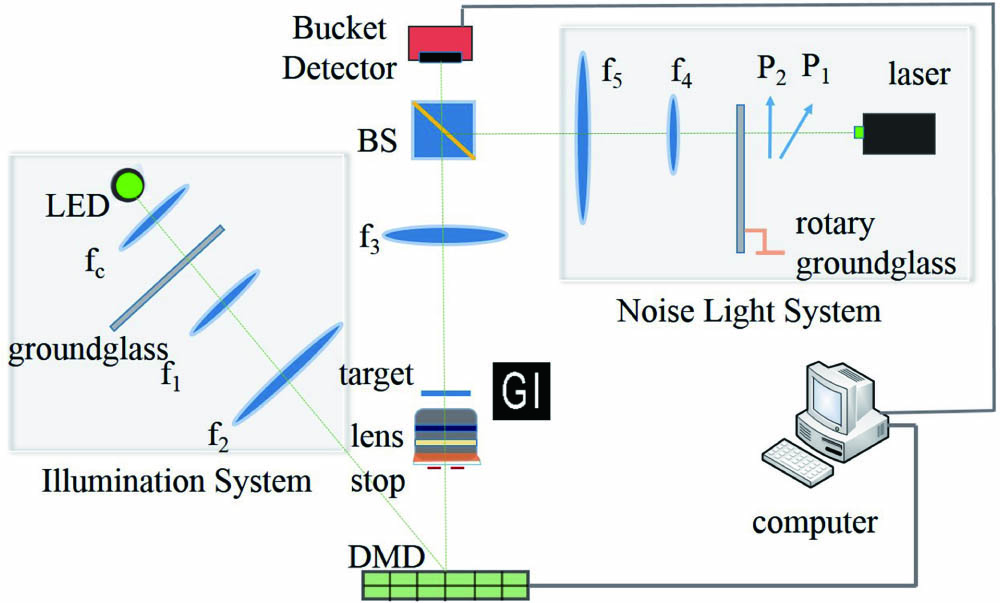
    To investigate the influence of the sparsity of speckle patterns on the quality of GI, the experimental system is established and shown in Fig. 1. The system consists of two parts: signal light path and noise light path. In the signal light path, thermal light emitted from a green naked bulk LED (Thorlabs, M530L3) is collimated by a short focal length lens fc with focal length of 50 mm and diameter of 25.4 mm to make the DMD window fully illuminated. A stationary ground glass disk and the adjacent Kohler illumination system consisting of two lenses, with focal lengths of 150 mm and 100 mm, are used to generate a uniform illumination on the DMD. By combining each set of 8×8 pixels into a single resolution cell, 512×512 pixels from the center of the DMD are chosen to produce a 64×64 pattern I64×64s, where each resolution element takes the value of 0 or 1, and s denotes the sth pattern.

    Experimental setup of the influence of the sparsity of random speckle illumination on GI.

    Figure 1.Experimental setup of the influence of the sparsity of random speckle illumination on GI.

    The patterns on the DMD are imaged to the object plane by a commercial lens (Cannon, EF-s 55-250). A stop placed in front of the commercial lens is utilized to control the illumination energy. The object is a transmissive target consisting of two letters ‘GI’ and with 25 mm distance from the commercial lens. After passing through the object, the signal light is imaged to a bucket detector by f3 with focal length 100 mm through a 4f system. In the noise light path, pseudothermal light generated by a 532 nm continuous laser and a rotary ground glass passes through a Kohler system (consisting of f4 and f5, the focal lengths are 25 mm and 100 mm, respectively) and enters the receiving system after the beam splitter (BS). A pair of polarizers (P1, P2) is placed between the laser and rotary ground glass to control the power of the noise light. It should be pointed out that the diameter of the noise light emitted from the laser is 1.5 mm, and the distance between f4 and the rotary ground glass is 150 mm. Lens f5 expands two times the speckles on f4 and images them onto the bucket detector.

    The patterns used in this work are drawn from random Bernoulli distribution B(0,1). For the k-sparse patterns, there are k elements, whose values are one, and the other elements are zero. The sparsity of the pattern is defined as β=kN,where N is the number of elements in each pattern. and N=m×n. Because k-sparse patterns are pre-loaded by the DMD, there is no reference path.

    In the framework of GI, the transmission OGI of the object can be reconstructed by computing the intensity fluctuation correlation between the intensity distribution of the reference patterns I64×64s and the bucket signal intensities Bs recorded by the bucket detector: OGI=1Ks=1K(IsIs)(BsBs),where K is the total measurement number and stays unchanged throughout the GI experiment, stands for ensemble averaging, and Is=1Ks=1KIs represents the ensemble average of Is. Bs=αIsO(x,y)dxdy+ns, α is a factor, which takes into account the loss in the signal light path, O(x,y) is the transmission function of the object, and ns denotes the noise introduced to the bucket detector by the noise light path. Bs can be equivalently expressed as Bs=αIs[O(x,y)+ε(x,y)]dxdy, where αIsε(x,y)dxdy=ns. It needs pointing out that ε(x,y) is a phenomenological representation of the noise term ns on the target plane.

    After some derivation following Ref. [22], Eq. (2) can be expressed in a form of matrix OGI=αKMC(T+ε),where MC is the matrix that measures the properties of reference patterns Irs, and MC=(AIA)T(AIA).

    Here, A denotes the measurement matrix, and each row of A is reshaped from Is(m,n), which makes A a K×N matrix. I is a K×N matrix whose elements are all 1. T is the ground truth of the object. ε denotes the noise introduced to the bucket detector, and ε is reshaped from ε(x,y). It needs to be noted that MC is the Gram matrix of the zero mean matrix (AIA). It is obvious that the more the matrix MC is similar to an identity matrix, the better the imaging quality for measurement matrix A is. Therefore, following the work of Ref. [22], grayscale fidelity γ is introduced to evaluate the character of measuring matrix: γ=N*MC(i,i)0[MC(i,i)1]2,where N* denotes the total number of nonzero diagonal elements of MC. When the diagonal element is zero, the image information of the corresponding pixel is lost. From Eq. (3), A alone cannot evaluate the imaging quality of GI, and the noise term that exists in the bucket signal should be considered.

    For the GISC method, the gradient projection for sparse reconstruction algorithm GISC is used[24]. The transmission O(x,y) of the object can be reconstructed by solving the optimization program, OGISC=|O|,which minimizes:12YAO22+τO1,where O denotes the retrieved image, τ denotes a non-negative parameter, 2 denotes the l2 norm, 1 denotes the l1-norm, and Y denotes the bucket signal.

    In the theory of GISC, the mutual coherence of columns of the measurement matrix is recognized as an important index to evaluate the reconstruction quality of the measurement matrix: μ=maxij|Ai,Aj|Ai2Aj2,where x,y denotes the inner product of the vectors x and y, and Ai is the ith column of the matrix A.

    3. Experimental Results

    To investigate the imaging performance of GI and GISC under different sparsity of patterns with different noise levels, the concrete parameters in the experiments are set as follows: the object size is 6 mm, and the minimum width of the object is about 1 mm. The DMD exposure time is 40 ms, and the bucket detector exposure time is set as 80 μs. The noise light power after two polarizers is selected to be 0 mW, 0.1 mW, 0.6 mW, and 3 mW. The sparsity of patterns is {1, 64, 512, 2048, 3584, 4032, 4095}/4096. The measurement number for GI is a full sampling number at 4096, while it is 3000 for GISC to examine the compressive sampling of GISC.

    The experimental results are shown in Fig. 2. It shows that imaging performances of GI and GISC improve as the sparsity of patterns approaches 0.5. When sparsity β exceeds 0.5, the imaging quality for both GI and GISC decreases with the increase of β. GISC is better than GI when the noise is not heavy. However, GISC is worse than GI when the noise is heavy. The phenomenon can be explained by Eq. (5) in Ref. [25], and GISC is more sensitive to noise compared with GI. From Figs. 2(a)2(c), it indicates that the imaging quality of GI will not improve much when the sparsity of matrix A increases, which means that the sparser source still results in satisfying imaging quality. This may lead to a simpler, faster, and cheaper GI system, especially in some waveband in which the independent random modulated element is difficult to manufacture.

    Experimental results of GI and GISC under different noise levels. (a)–(d) are imaging results of GI under 0 mW, 0.1 mW, 0.6 mW, and 3 mW noise light power, respectively; (e)–(h) are imaging results of GISC under 0 mW, 0.1 mW, 0.6 mW, and 3 mW noise light power, respectively. From top to bottom, (i)–(vii) represent the sparsity of {1, 64, 512, 2048, 3584, 4032, 4095}/4096, respectively.

    Figure 2.Experimental results of GI and GISC under different noise levels. (a)–(d) are imaging results of GI under 0 mW, 0.1 mW, 0.6 mW, and 3 mW noise light power, respectively; (e)–(h) are imaging results of GISC under 0 mW, 0.1 mW, 0.6 mW, and 3 mW noise light power, respectively. From top to bottom, (i)–(vii) represent the sparsity of {1, 64, 512, 2048, 3584, 4032, 4095}/4096, respectively.

    To evaluate the quality of reconstructed images, the structural similarity (SSIM) index is introduced[26], which is more suitable for the human eye compared with the peak SNR in this case. Assuming the measured object is X, and the reconstructed image is Y, the SSIM index of the two images can be determined: SSIM(X,Y)=(2μXμY+c1)(2σXY+c2)(μX2+μY2+c1)(σX2+σY2+c2),where μX is the mean value of X, μY is the mean value of Y, σX is the variance of X, σY is the variance of Y, σXY is the covariance of X and Y, c1=(k1L)2 and c2=(k2L)2 are constants used to maintain stability, L is the dynamic range of pixel values, k1=0.01, k2=0.03, and L=255. Figure 3 shows the SSIM curves of the reconstructed image with varying sparsity of patterns. The range of SSIM varies from 0 (when two images are different) to 1 (when two images are the same). It can be clearly observed that the SSIM of GI/GISC obtains the greatest value when the sparsity is 0.5 under a fixed noisy light level and decreases as the sparsity deviates from 0.5.

    SSIM of GI and GISC under different noisy light levels. (a) and (b) are SSIM of GI and GISC versus sparsity of patterns, respectively.

    Figure 3.SSIM of GI and GISC under different noisy light levels. (a) and (b) are SSIM of GI and GISC versus sparsity of patterns, respectively.

    In order to explain the results of GI and GISC shown in Figs. 2 and 3, detection SNR (DSNR) and some characteristics of the measurement matrix A are analyzed. Based on the knowledge of GI and GISC, the DSNR of GI is defined as the ratio of the bucket signal fluctuation and the noise light fluctuation, and the DSNR of GISC is defined as the ratio of the bucket signal mean value and the noise light fluctuation: DSNRGI=10log10std(Y)std(Noise),DSNRGISC=10log10mean(Y)std(Noise),where std() denotes standard deviation. The bucket signal when the noise light power is 0 mW is taken as the signal Y, and the Noise term is obtained by calculating the difference between the signal Y and the bucket signal when the noise light power is 0.1 mW, 0.6 mW, and 3 mW.

    The theoretical analysis of measurement matrix A according to Eq. (5) and the experimental DSNR of GI are shown in Fig. 4. In Fig. 4(a), the grayscale fidelity γ reaches its maximum when the sparsity β is 0.5. γ drops sharply when β is larger than 0.8 or smaller than 0.2. In Fig. 4(b), DSNRGI has its biggest value when the sparsity is 0.5, and the DSNRGI declines rapidly when β is larger than 0.8 or smaller than 0.2 for a fixed noise level. Through Figs. 4(a) and 4(b), it shows that, in the framework of GI, sparsity makes the measurement matrix performance and DSNR change synchronously when noise is in the same level. These two factors together influence the imaging quality, which is consistent with the experimental results shown in Figs. 2(a)2(d) and 3(a). When β gets off 0.5, both γ and DSNRGI decrease, resulting in the degradation of imaging quality. A large γ value and high DSNR improve imaging quality in GI.

    Analysis result of GI. (a) The curve of grayscale fidelity γ; (b) the curves of DSNR under different noise levels.

    Figure 4.Analysis result of GI. (a) The curve of grayscale fidelity γ; (b) the curves of DSNR under different noise levels.

    The theoretical analysis of measurement matrix A according to Eq. (7) and the experimental DSNR of GISC are shown in Fig. 5. In Fig. 5(a), the mutual coherence μ increases almost linearly as the sparsity β ranges from 0.2 to 0.9, and μ reaches its maximum when β is about 1. Generally, a small μ guarantees a better reconstruction quality in compressed sensing (CS)[27]. However, it shows that the reconstruction performance does not improve when β is smaller than 0.5 in Figs. 2(e)2(h) and 3(b), which obviously violates the intuition. It directly shows that the characteristic of the measurement matrix cannot exclusively determine the imaging quality in GISC. In Fig. 5, DSNRGISC increases as β grows. However, the imaging quality does not. In the circumstance of GISC, it illustrates that either small μ or large DSNR alone cannot ensure a satisfying reconstructed image. It is the combination of the measurement matrix and DSNR that dominates the imaging quality of GISC.

    Analysis result of GISC. (a) The curve of mutual coherence μ; (b) the curves of DSNR under different noise levels.

    Figure 5.Analysis result of GISC. (a) The curve of mutual coherence μ; (b) the curves of DSNR under different noise levels.

    4. Conclusion

    In conclusion, we have investigated the influence of the sparsity of random speckle illumination on GI under different noise levels. The sparsity 0.5 is the best for GI and GISC. The DSNR of the bucket signal or the characteristic of the measurement matrix alone cannot be recognized as the exclusive factor that dominates the imaging quality. It surely happens that, in GISC, a bigger DSNR may accompany a worse imaging quality when the measurement matrix has a larger μ. The measurement matrix characterisitic should be considered together with DSNR to evaluate reconstruction performance. We believe this work may promote practical application for GI via an array source.

    References

    [1] R. S. Bennink, S. J. Bentley, R. W. Boyd, J. C. Howell. Quantum and classical coincidence imaging. Phys. Rev. Lett., 92, 033601(2004).

    [2] J. Cheng, S. Han. Incoherent coincidence imaging and its applicability in X-ray diffraction. Phys. Rev. Lett., 92, 093903(2004).

    [3] D.-Z. Cao, J. Xiong, K. Wang. Geometrical optics in correlated imaging systems. Phys. Rev. A, 71, 013801(2005).

    [4] D. Zhang, Y.-H. Zhai, L.-A. Wu, X.-H. Chen. Correlated two-photon imaging with true thermal light. Opt. Lett., 30, 2354(2005).

    [5] M. D’Angelo, Y. Shih. Quantum imaging. Laser Phys. Lett., 2, 567(2005).

    [6] J. H. Shapiro, R. W. Boyd. The physics of ghost imaging. Quantum Inf. Process., 11, 949(2012).

    [7] H. Guo, R. He, C. Wei, Z. Lin, L. Wang, S. Zhao. Compressed ghost edge imaging. Chin. Opt. Lett., 17, 071101(2019).

    [8] G. Wang, H. Zheng, Z. Tang, Y. He, Y. Zhou, H. Chen, J. Liu, Y. Yuan, F. Li, Z. Xu. Naked-eye ghost imaging via photoelectric feedback. Chin. Opt. Lett., 18, 091101(2020).

    [9] A. D. Rodríguez, P. Clemente, E. Irles, E. Tajahuerce, J. Lancis. Resolution analysis in computational imaging with patterned illumination and bucket detection. Opt. Lett., 39, 3888(2014).

    [10] S. M. Mahdi Khamoushi, Y. Nosrati, S. Hassan Tavassoli. Sinusoidal ghost imaging. Opt. Lett., 40, 3452(2015).

    [11] Z. Zhang, X. Ma, J. Zhong. Single-pixel imaging by means of Fourier spectrum acquisition. Nat. Commun., 6, 6225(2015).

    [12] C. Zhou, T. Tian, C. Gao, W. Gong. Multi-resolution progressive computational ghost imaging. J. Opt., 21, 055702(2019).

    [13] J. Cheng. Ghost imaging through turbulent atmosphere. Opt. Express, 17, 7916(2009).

    [14] W. Gong, S. Han. Correlated imaging in scattering media. Opt. Lett., 36, 394(2011).

    [15] M. Bina, D. Magatti, M. Molteni, A. Gatti, L. Lugiato, F. Ferri. Backscattering differential ghost imaging in turbid media. Phys. Rev. Lett., 110, 083901(2013).

    [16] C. Zhao, W. Gong, M. Chen, E. Li, H. Wang, W. Xu, S. Han. Ghost imaging lidar via sparsity constraints. Appl. Phys. Lett., 101, 141123(2012).

    [17] B. I. Erkmen. Computational ghost imaging for remote sensing. J. Opt. Soc. Am. A, 29, 782(2012).

    [18] O. Katz, Y. Bromberg, Y. Silberberg. Compressive ghost imaging. Appl. Phys. Lett., 95, 131110(2009).

    [19] W. Gong, S. Han. High-resolution far-field ghost imaging via sparsity constraint. Sci. Rep., 5, 9280(2015).

    [20] B. Sun, M. P. Edgar, R. Bowman, L. E. Vittert, S. Welsh, A. Bowman, M. J. Padgett. 3D computational imaging with single-pixel detectors. Science, 340, 844(2013).

    [21] J. Chen, W. Gong, S. Han. Sub-Rayleigh ghost imaging via sparsity constraints based on a digital micro-mirror device. Phys. Lett. A, 377, 1844(2013).

    [22] C. Wang, W. Gong, X. Shao, S. Han. The influence of the property of random coded patterns on fluctuation-correlation ghost imaging. J. Opt., 18, 065703(2016).

    [23] X. Liu, J. Shi, X. Wu, G. Zeng. Fast first-photon ghost imaging. Sci. Rep., 8, 5012(2018).

    [24] R. Gribonval, M. Nielsen. Sparse representations in unions of bases. IEEE Trans. Inform. Theory, 49, 3320(2003).

    [25] E. J. Candès, J. K. Romberg, T. Tao. Stable signal recovery from incomplete and inaccurate measurements. Commun. Pur. Appl. Math., 59, 1207(2006).

    [26] Z. Wang, E. P. Simoncelli, A. C. Bovik. Multiscale structural similarity for image quality assessment. 37th Asilomar Conference on Signals, Systems and Computers, 1398(2003).

    [27] D. L. Donoho, M. Elad, V. N. Temlyakov. Stable recovery of sparse overcomplete representations in the presence of noise. IEEE Trans. Inform. Theory, 52, 618(2006).

    Long Pan, Chenjin Deng, Cuiping Yu, Shuai Yue, Wenlin Gong, Shensheng Han. Influence of the sparsity of random speckle illumination on ghost imaging in a noise environment[J]. Chinese Optics Letters, 2021, 19(4): 041103
    Download Citation