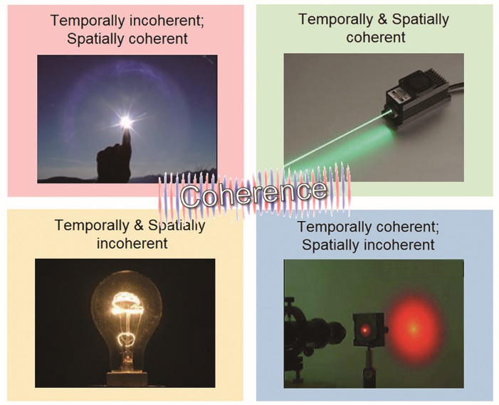
Fig. 1. Several typical examples of light sources with different degrees of temporal coherence and spatial coherence

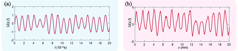
Fig. 2. Representation of optical signal in time and space. (a) Optical signal is a function of time at a certain point in space; (b) optical signal is a function of space at a certain point in time

Fig. 3. Superposition of light waves with different frequencies. (a) Waves with different frequencies are coherently superimposed into one pulse wave packet; (b) waves with different frequencies are incoherently superimposed into one continuous wave (non-periodic and infinite width), and its phase and amplitude vary randomly

Fig. 4. Basic principle of Fourier transform spectrometer

Fig. 5. Michelson stellar interferometer measures the spatial coherence of a quasi-monochromatic wave field by interferometry to infer the size of the light source. (a) Optical configuration; (b) photograph of a real system

Fig. 6. Relationship between classical coherence theory and phase space optics

Fig. 7. Characterization of common signal transformations in phase space. (a) Fresnel propagation; (b) Chirp modulation (lens); (c) Fourier transform; (d) fractional Fourier transform; (e) magnifier

Fig. 8. Wigner distribution function of special signals. (a) Point source; (b) plane wave; (c) spherical wave; (d) phase slow-varying wave; (e) Gaussian signal

Fig. 9. Parameterization of the light field. (a) Seven-dimensional plenoptic function; (b) two planes parameterization of four-dimensional light field; (c) position-angular parameterization of four-dimensional light field

Fig. 10. Relationship between Wigner distribution function and light field of a smooth coherent wavefront. Phase is represented as the localized spatial frequency (instantaneous frequency) in the Wigner distribution function. Rays travel perpendicularly to the wavefront (phase normal) ^[128]. (a) Wavefront in real space; (b) Wigner distribution function in phase space; (c) light field in position-angle space

Fig. 11. Classification of phase imaging techniques

Fig. 12. Classification of the coherence measurement techniques

Fig. 13. Young’s interferometry with two holes^[22]

Fig. 14. Reversed-wavefront Young’ interferometry^[77]

Fig. 15. Distributions of nonredundant array method and experimental scheme^[78]. (a1) Superior in points on axes; (a2) central distribution of points; (a3) superior in points out of axes; (b) experimental scheme of nonredundant array method

Fig. 16. Experimental scheme of self-referencing interferometry^[80]

Fig. 17. Correspondence between Wigner distribution function and ambiguity function

Fig. 18. Basic principle of phase space tomography. (a) Vertical projection; (b) quarter rotation projection; (c) rotation by 90° projection; (d) superposition of all projections from different angles

Fig. 19. Two different transformations of WDF for phase space tomography. (a) WDF of complex signal; (b) WDF after Fresnel diffraction; (c) phase space WDF after fractional Fourier transform; (d) correspondence between Fresnel diffraction and fractional Fourier transform

Fig. 20. Optical path structure of phase space tomography^[85]

Fig. 21. Experimental device for measuring spatial coherence based on edge diffraction^[84]

Fig. 22. Direct phase space measurement. (a) Direct phase space measurement based on pinhole scanning; (b) direct phase space measurement based on microlens array

Fig. 23. Schematic of a simplistic view of coherent field and partially (spatially) coherent field. (a) A coherent field requires a 2D complex amplitude representation, the surface of the constant phase is interpreted as wavefronts with geometric light rays traveling normal to them; (b) a partially coherent field requires a 4D coherence function to accurately represent its properties such as propagation and diffraction. The “phase” (generalized phase) of a partially coherent light field is the statistical average of phases (spatial frequency, direction of propagation) at each position in space

Fig. 24. Principle of the Shack-Hartmann sensor and light field camera. (a) For coherent field, the Shack-Hartmann sensor forms a focus spot array sensor signal; (b) for partially coherent field, the Shack-Hartmann sensor forms an extended source array sensor signal; (c) for incoherent imaging, the light field camera produces a 2D sub-aperture image array

Fig. 25. Classification of light field imaging techniques

Fig. 26. Light field capture based on camera arrays. (a) Light field gantry^[126]; (b) large camera arrays^[110]; (c) micro light field acquisition acquired by the 5×5 camera array system^[189]

Fig. 27. Various light field cameras based on microlens array

Fig. 28. Computational light field imaging based on coded mask. (a) Light field acquisition of mask enhanced camera^[191]; (b) light field acquisition of compressive photography^[192]

Fig. 29. Light field imaging based on programmable aperture. (a) Programmable aperture light field camera^[104]; (b) programmable aperture light field microscope^[106]

Fig. 30. Light field representation of a slowly varying object under spatially stationary illumination^[128]

Fig. 31. Light field microscope model. (a) Traditional bright field microscope; (b) light field microscope^[111]; (c) light field microscopic model based on wave optics theory^[112]; (d) Fourier light field microscope^[113]

Fig. 32. Comparison between TIE and WOTF^[207]. (a1)(b1) Physical implications of TIE and WOTF; (a2)(b2) geometric illustrations for deriving the PGTF and WOTF; (a3)(b3) PGTF and WOTF for phase imaging under different s

Fig. 33. Direct visualization of coherent images reconstructed from coherent holograms^[209]

Fig. 34. Photon correlation holography^[213]. (a) Concept diagram of photon-dependent holography; (b) schematic diagram of intensity interferometer

Fig. 35. Representative optical setup for incoherent holography. (a) Optical path of modified triangular interferometer^[217]; (b) optical path of FINCH^[214]; (c) Michelson interferometer^[119]; (d) Sagnac interferometer^[215]; (e) Mach-Zehnder interferometer^[216,218]

Fig. 36. Typical imaging optical path for COACH. (a) Structure of COACH^[115]; (b) structure of I-COACH^[117]; (c) structure of LI-COACH^[116]

Fig. 37. Schematic of non-invasive scattering imaging through strong scattering layers^[237]

Fig. 38. Single frame imaging based on speckle autocorrelation through strong scattering layer^[238]. (a) Experimental setup; (b) raw camera image; (c) autocorrelation; (d) image reconstructed by an iterative phase-retrieval algorithm; (e) photograph of the experiment; (f) raw camera image; (g)--(k) Left column is calculated autocorrelation, middle column is reconstructed object; right column is image of the real object

Fig. 39. Conventional incoherent synthetic aperture structure. (a) Michelson interferometer; (b) common secondary structure; (c) multiple telescopes structure

Fig. 40. Design model of the initial generation of SPIDER imaging conceptual system. (a) Explosive view of SPIDER; (b) PIC schematics of the two physical baselines and three spectral bands; (c) arrangement of SPIDER microlens; (d) corresponding frequency-spectrum coverage

Fig. 41. Incoherent synthetic aperture technology based on FINCH^[243]

Fig. 42. RSI of visible cone-beam tomography^[79]

Fig. 43. Application of light field microscopy in bioscience.(a) Mouse with a head-mounted MiniLFM^[252]; (b) imaging Golgi-derived membrane vesicles in living COS-7 cells using HR-LFM ^[74]; (c) dynamics during neutrophil migration in mouse liver using DAOSLIMIT^[73]; (d) hunting activity of zebrafish and the neural activity of mouse brain observed by confocal light field microscope^[75]

Fig. 44. Microscopy imaging based on FINCH. (a) FINCHSCOPE schematic; (b) FINCHSCOPE fluorescence sections of pollen grains^[118]; (c) wide-field image and reconstructed FINCH image of pollen grains captured using a 20×(0.75 NA) objective^[253]; (d) comparative imaging of three different Golgi apparatus proteins in HeLa cells using wide-field (left) and FINCH(right)^[255]

Fig. 45. Light field imaging in computational photography. (a) Light field refocusing^[101]; (b) synthetic aperture imaging based on light field^[259]

Fig. 46. Computational photography refocusing based on FINCH. (a) Digital refocusing based on FINCH^[214]; (b) colorful digital holography refocusing^[260]; (c) full color holographic digital refocusing under natural light illumination^[119]

Fig. 47. X-ray characterization via phase space tomography. (a) Measured intensity distribution of the X rays as a function of lateral position and along the direction of propagation^[263]; (b) phase space density reconstructed from the data in Fig.47(a); (c)(d) measured complex degree of coherence for the beams in the two conditions ^[263]

Fig. 48. Optical beam characterization via phase space tomography. (a) 1D signal^[265]; (b) optical beams separable in Cartesian coordinates^[264]; (c) rotationally symmetric beams^[266]; (d) intensity distributions of the test beams with different degrees of coherence (first row), the Wigner distribution function of the beams exhibits hidden differences associated with their coherence state (second row)^[267]

Fig. 49. Schematic diagram of phase retrieval and factor M² calculation^[268]. (a)(b) Axial intensity images at two different longitudinal positions; (c) phase retrieval by TIE; (d) reconstructed intensity distribution at any selected plane; (e) performing a hyperbolic fit to the beam widths and calculating the M²

Fig. 50. Under different numerical apertures, the phase is recovered directly through the gravity of the light field^[128]. (a) 0.05; (b) 0.15; (c) 0.2; (d) 0.25

Fig. 51. Reconstructed phases with and without mode decomposition method under partially coherent illumination^[269]

Fig. 52. Stack imaging based on coherent mode decomposition. (a) Decoherence in scattering imaging^[270];(b) experimental scheme of Fourier stack imaging with single-mode and multi-mode multiplexing^[271]

Fig. 53. Synthetic aperture technique based on FINCH. (a)--(c) Three phase functions loaded on SLM; (d) single aperture reconstruction result; (e) synthetic multi aperture reconstruction result^[243]; (f) image obtained by the conventional imaging system; (g) reconstructed image corresponding to the hologram produced by the 360×360 FINCH system; (h) reconstructed image corresponding to the hologram produced by synthetic aperture of double lens FINCH; (i) reconstructed image corresponding to the hologram produced by the 1080×1080 FINCH system^[275]

Fig. 54. Experimental results of SPIDER imaging^[277]. (a) PIC image experimental platform; (b) iterative image reconstruction result of Fig.54(g); (c)(g) two images of the target; (d)(h) corresponding principle simulation results of target image; (e)(i) imaging results obtained by inverse Fourier transform reconstruction; (f)(j) after correcting the swing error of the turntable, the imaging results are reconstructed by inverse Fourier transform

Fig. 55. Lensless noninterference coded aperture dependent holography^[116]. (a) Two LEDs; (b) two one-dime coins

Fig. 56. Incoherent lensless imaging based on Fresnel region aperture. (a) Real time image capture and reconstruction of lens less camera^[279]; (b) binary, gray, and color images are reconstructed by Fresnel region aperture single frame lensless camera^[282]

Table 1. Coherence measurement: classical coherence theory and phase space optics theory

Table 2. Properties of Wigner distribution function

Table 3. Common optical transformation of Wigner distribution function

Table 4. Spatial and phase space characterization of common optical signals

Table 5. Optical field transmission: from coherent to partially coherent