• Photonics Research
  • Vol. 10, Issue 2, 303 (2022)
He Cheng1, Pooria Golvari2, Chun Xia1、2, Mingman Sun3, Meng Zhang3, Stephen M. Kuebler1、2、4, and Xiaoming Yu1、*
Author Affiliations
  • 1CREOL, The College of Optics and Photonics, University of Central Florida, Orlando, Florida 32816, USA
  • 2Department of Chemistry, University of Central Florida, Orlando, Florida 32816, USA
  • 3Department of Industrial and Manufacturing Systems Engineering, Kansas State University, Manhattan, Kansas 66506, USA
  • 4Department of Material Science and Engineering, University of Central Florida, Orlando, Florida 32816, USA
  • show less
    DOI: 10.1364/PRJ.439592 Cite this Article Set citation alerts
    He Cheng, Pooria Golvari, Chun Xia, Mingman Sun, Meng Zhang, Stephen M. Kuebler, Xiaoming Yu. High-throughput microfabrication of axially tunable helices[J]. Photonics Research, 2022, 10(2): 303 Copy Citation Text show less
    High-throughput microfabrication of helical structures using self-accelerating beams (SABs). (a) Experimental setup: BBO, beta barium borate crystal; PBS, polarizing beam splitter; BE, beam expander; BS, non-polarizing beam splitter; SLM, spatial light modulator; M, mirror; L, lens; ID, iris diaphragm; Obj, objective lens; CMOS, complementary metal–oxide-semiconductor. (b) Calculation of a computer-generated hologram (CGH). Phase order l=−10, m=−9. (c) Illustration of exposure in the SU-8 sample. Green arrow shows the beam propagation direction. (d) Fourier spectrum of an SAB at the Fourier plane of the 4-f system. The white dashed circle represents the iris diaphragm acting as a low-pass filter to isolate the zeroth-order beam. (e) Simulation of iso-intensity and x-y intensity distribution of an SAB in SU-8. (f) SEM images of fabricated helices, including a 45° view of a 30×30 matrix (individual helix highlighted in yellow, scale bar corresponds to 30 μm.). The white-boxed inset shows a high-magnification view of a single helix.
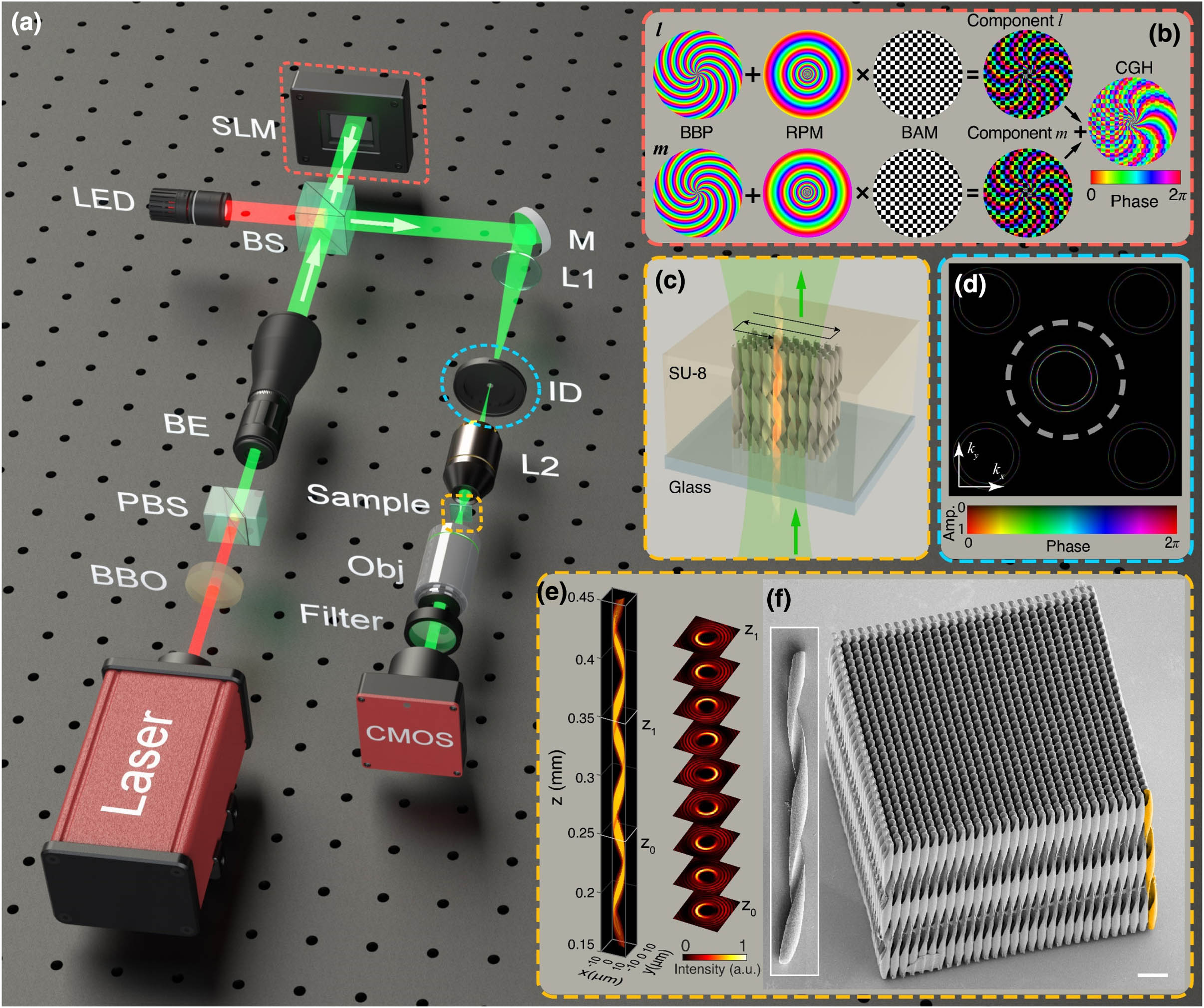
    Fig. 1. High-throughput microfabrication of helical structures using self-accelerating beams (SABs). (a) Experimental setup: BBO, beta barium borate crystal; PBS, polarizing beam splitter; BE, beam expander; BS, non-polarizing beam splitter; SLM, spatial light modulator; M, mirror; L, lens; ID, iris diaphragm; Obj, objective lens; CMOS, complementary metal–oxide-semiconductor. (b) Calculation of a computer-generated hologram (CGH). Phase order l=10, m=9. (c) Illustration of exposure in the SU-8 sample. Green arrow shows the beam propagation direction. (d) Fourier spectrum of an SAB at the Fourier plane of the 4-f system. The white dashed circle represents the iris diaphragm acting as a low-pass filter to isolate the zeroth-order beam. (e) Simulation of iso-intensity and x-y intensity distribution of an SAB in SU-8. (f) SEM images of fabricated helices, including a 45° view of a 30×30 matrix (individual helix highlighted in yellow, scale bar corresponds to 30 μm.). The white-boxed inset shows a high-magnification view of a single helix.
    Comparison of simulated and measured helical beams with (a)–(d) constant and (e)–(h) decelerated rotation rate. Phase order l=−10 and m=−9. (a), (e) Iso-intensity contours of simulated SABs in air. The threshold intensity (normalized) is set to 0.5. (b), (f) Simulated and (c), (g) measured x-y intensity distribution. Scale bar represents 5 μm. (d), (h) Rotation rate ω along optical axis. Red curves, designed profiles; orange points, measured data; blue dots, simulation results.
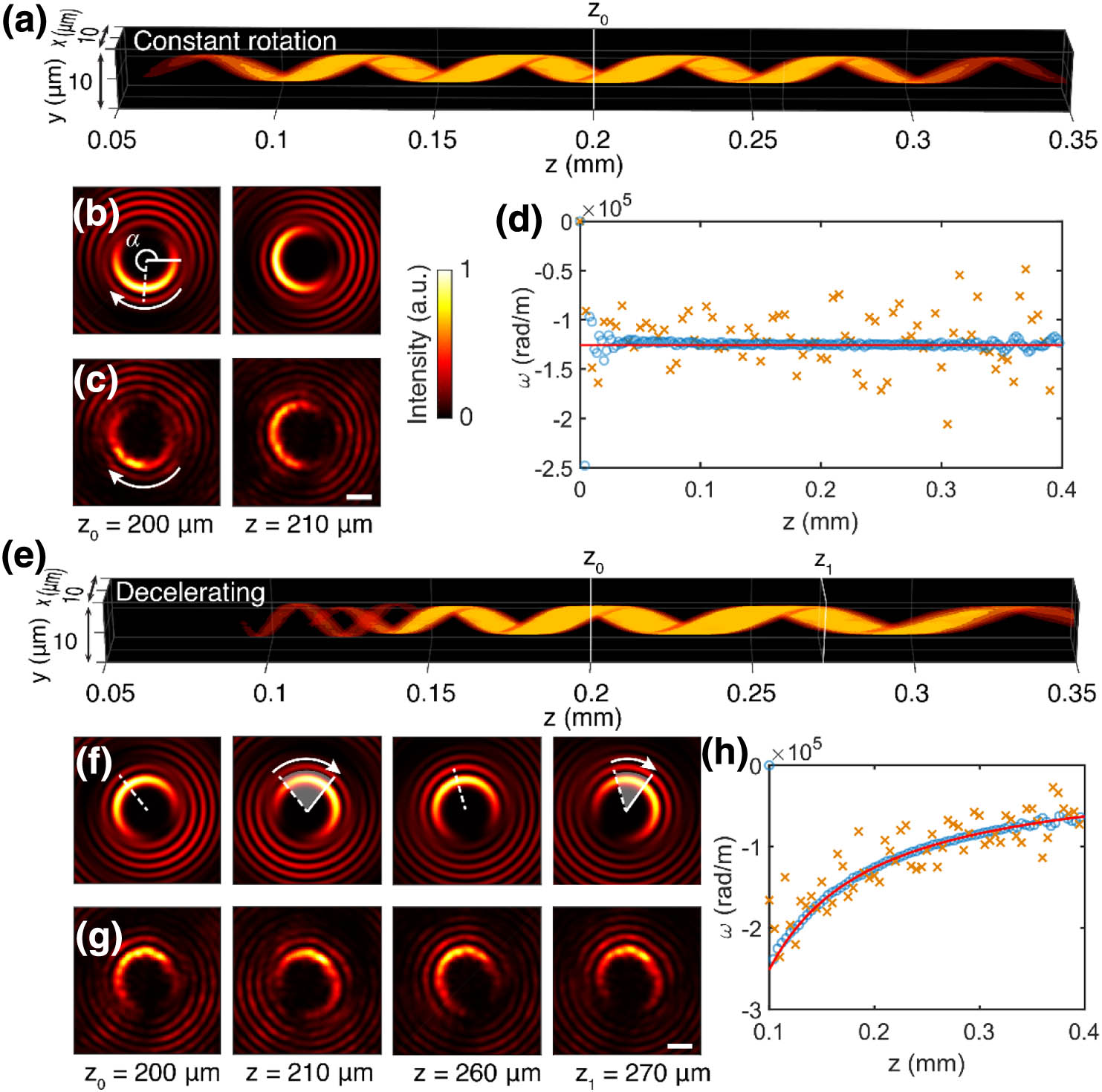
    Fig. 2. Comparison of simulated and measured helical beams with (a)–(d) constant and (e)–(h) decelerated rotation rate. Phase order l=10 and m=9. (a), (e) Iso-intensity contours of simulated SABs in air. The threshold intensity (normalized) is set to 0.5. (b), (f) Simulated and (c), (g) measured x-y intensity distribution. Scale bar represents 5 μm. (d), (h) Rotation rate ω along optical axis. Red curves, designed profiles; orange points, measured data; blue dots, simulation results.
    Comparison between helical beams simulated in SU-8 and fabrication results obtained with five SABs having different types of rotation. The contrast of each SEM image was adjusted individually to improve visibility and aid comparison. Scale bar corresponds to 20 μm.
    Fig. 3. Comparison between helical beams simulated in SU-8 and fabrication results obtained with five SABs having different types of rotation. The contrast of each SEM image was adjusted individually to improve visibility and aid comparison. Scale bar corresponds to 20 μm.
    Characterization of a fabricated helix. (a) SEM image of the helix with one edge highlighted. (b) One edge (red solid curve) of the helix is extracted from the optical microscopic image, and the distance d from the optical axis (white dotted-dashed line) is measured. Scale bar corresponds to 10 μm. (c) Comparison of d between measurement (orange triangle) and theoretical prediction (blue curve). Error bars represent ± one standard deviation.
    Fig. 4. Characterization of a fabricated helix. (a) SEM image of the helix with one edge highlighted. (b) One edge (red solid curve) of the helix is extracted from the optical microscopic image, and the distance d from the optical axis (white dotted-dashed line) is measured. Scale bar corresponds to 10 μm. (c) Comparison of d between measurement (orange triangle) and theoretical prediction (blue curve). Error bars represent ± one standard deviation.
    Matrices of various helical structures fabricated by a combination of exposure and linear translation.
    Fig. 5. Matrices of various helical structures fabricated by a combination of exposure and linear translation.
    Propagation model used in the derivation.
    Fig. 6. Propagation model used in the derivation.
    Simulation results of two beams with (a) large and (b) small helical diameters generated by changing the phase order (l,m). The transverse intensity profiles shown on the left are obtained at z=0.2 mm. Scale bar, 5 μm.
    Fig. 7. Simulation results of two beams with (a) large and (b) small helical diameters generated by changing the phase order (l,m). The transverse intensity profiles shown on the left are obtained at z=0.2  mm. Scale bar, 5 μm.
    Schematic for the propagation of helical beams into photoresist. L2 is the second lens of the 4-f system. Variable n is the refractive index of the photoresist, and z is the coordinate along the optical axis.
    Fig. 8. Schematic for the propagation of helical beams into photoresist. L2 is the second lens of the 4-f system. Variable n is the refractive index of the photoresist, and z is the coordinate along the optical axis.
    (a) Theory and (b) simulation of intensity distribution on the x-z plane of an SAB with a decelerating rotation rate propagating from air to the photoresist. White dashed lines indicate the interface between the two media. (c) Rotation rate ω at different z locations. Solid line is from Eq. (C6). Open circles are from the simulation. Discrepancies at small z are due to limitations of the algorithm used to extract ω for low intensities.
    Fig. 9. (a) Theory and (b) simulation of intensity distribution on the x-z plane of an SAB with a decelerating rotation rate propagating from air to the photoresist. White dashed lines indicate the interface between the two media. (c) Rotation rate ω at different z locations. Solid line is from Eq. (C6). Open circles are from the simulation. Discrepancies at small z are due to limitations of the algorithm used to extract ω for low intensities.
    Characterization of a fabricated helix from an SEM image. (a) Original image. (b) The edges are detected from the image by edge-detection algorithms. (c) Noise is suppressed and only one edge is displayed. (d) Locations along the edge are plotted.
    Fig. 10. Characterization of a fabricated helix from an SEM image. (a) Original image. (b) The edges are detected from the image by edge-detection algorithms. (c) Noise is suppressed and only one edge is displayed. (d) Locations along the edge are plotted.
    Characterization of a fabricated helix from a transmissive optical microscopic image. Red curve overlayed on the image is used to illustrate the edge that is extracted.
    Fig. 11. Characterization of a fabricated helix from a transmissive optical microscopic image. Red curve overlayed on the image is used to illustrate the edge that is extracted.
    He Cheng, Pooria Golvari, Chun Xia, Mingman Sun, Meng Zhang, Stephen M. Kuebler, Xiaoming Yu. High-throughput microfabrication of axially tunable helices[J]. Photonics Research, 2022, 10(2): 303
    Download Citation