Steering paradox for Einstein–Podolsky–Rosen argument and its extended inequality

Tianfeng Feng; Changliang Ren; Qin Feng; Maolin Luo; Xiaogang Qiang; Jing-Ling Chen; Xiaoqi Zhou

doi:10.1364/PRJ.411033

Abstract

The Einstein–Podolsky–Rosen (EPR) paradox is one of the milestones in quantum foundations, arising from the lack of a local realistic description of quantum mechanics. The EPR paradox has stimulated an important concept of “quantum nonlocality,” which manifests itself in three types: quantum entanglement, quantum steering, and Bell’s nonlocality. Although Bell’s nonlocality is more often used to show “quantum nonlocality,” the original EPR paradox is essentially a steering paradox. In this work, we formulate the original EPR steering paradox into a contradiction equality, thus making it amenable to experimental verification. We perform an experimental test of the steering paradox in a two-qubit scenario. Furthermore, by starting from the steering paradox, we generate a generalized linear steering inequality and transform this inequality into a mathematically equivalent form, which is friendlier for experimental implementation, i.e., one may measure the observables only in the

x

y

, or

z

axis of the Bloch sphere, rather than other arbitrary directions. We also perform experiments to demonstrate this scheme. Within the experimental errors, the experimental results coincide with theoretical predictions. Our results deepen the understanding of quantum foundations and provide an efficient way to detect the steerability of quantum states.

Ψ (x_{1}, x_{2}) = \int_{- \infty}^{+ \infty} e^{i p (x_{1} - x_{2} + x_{0}) / ℏ} d p

Undoubtedly, the EPR paradox is a milestone in quantum foundations, as it has opened the door of “quantum nonlocality.” In 1964, Bell made a distinct response to the EPR paradox by showing that quantum entangled states may violate Bell’s inequality, which hold for any local-hidden-variable model [4]. This indicates that local-hidden-variable models cannot reproduce all quantum predictions, and the violation of Bell’s inequality by entangled states directly implies a kind of nonlocal property—Bell’s nonlocality. Since then, Bell’s nonlocality has achieved rapid and fruitful development in two directions [5]. (i) On one hand, more and more Bell’s inequalities have been introduced to detect Bell’s nonlocality in different physical systems, e.g., the Clause-Horne-Shimony-Holt (CHSH) inequality for two qubits [6], the Mermin-Ardehali-Belinskii-Klyshko (MABK) inequality for multipartite qubits [7], and the Collins-Gisin-Linden-Masser-Popescu inequality for two qudits [8]. (ii) On the other hand, some novel quantum paradoxes, or the all-versus-nothing (AVN) proofs, have been suggested to reveal Bell’s nonlocality without inequalities. Typical examples are the Greenberger-Horne-Zeilinger (GHZ) paradox [9] and the Hardy paradox [10]. Experimental verifications of Bell’s nonlocality have also been carried out; for instance, Aspect et al. successfully made the first observation of Bell’s nonlocality with the CHSH inequality [11], Pan et al. tested the three-qubit GHZ paradox in a photon-based experiment [12], and very recently, Luo et al. tested the generalized Hardy paradox for multi-qubit systems [13].

Sign up for Photonics Research TOC. Get the latest issue of Photonics Research delivered right to you！Sign up now

ρ_{AB} = | Ψ (α, ϕ) ⟩ ⟨ Ψ (α, φ) |

\hat{n}

k = 1

α \in (0, π / 2)

{\hat{x}, \hat{y}, \hat{z}}

σ_{x}

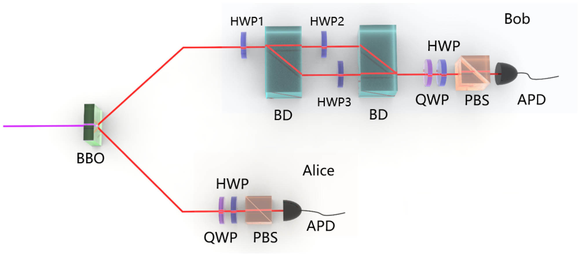
Figure 1.Experimental setup. Polarization-entangled photons pairs are generated via nonlinear crystal. An asymmetric loss interferometer along with half-wave plates (HWPs) is used to prepare two-qubit pure entangled states. The projective measurements are performed using wave plates and polarization beam splitter (PBS).

Figure 2.Experimental results for pure states. (a) Experimental results concerning the steering paradox “

2 = 1

.” The black and blue solid lines represent the quantum prediction

S \equiv P_{total}^{QM} = 2

and the classical bound

C = 1

based on the LHV models, respectively. The black cubes and the red lines show the experimental results with error bar. (b) Experimental results for the three-setting GLSI (7). The black and blue solid lines represent the quantum and classic bounds, respectively, which are obtained by maximizing the difference between

S_{3}^{'}

and

C_{LHS}^{'}

for any fixed

α

. The black (blue) dot line represents the quantum violation

⟨ S_{3}^{''} ⟩ = 1 + 2 \sin 2 α

(classical value

C = \sqrt{3}

) of the usual three-setting LSI (8). The red cubes are the experimental points for the inequality (7). The light yellow range is

α \in (0, (\arcsin \frac{\sqrt{3} - 1}{2}) / 2]

, where the LSI (8) cannot detect the steerability but the GLSI can. (c) Experimental violation for

α = \frac{π}{36}, \frac{π}{18}

| Ψ (α) ⟩

Figure 3.Experimental results for mixed states. (a), (b) Steering detection for the generalized Werner state

ρ_{1}

and the asymmetric mixed state

ρ_{2}

. The light purple and pink surfaces represent the quantum value and the classical bound of the GLSI (7), respectively. The black (blue) dots denote results for the quantum states that can (cannot) experimentally violate the GLSI (7). The zoom shows the area where steering cannot be detected by usual LSI (8), whereas GLSI may be useful.

k = 1

Recently, quantum steering has been applied to the one-sided device-independent quantum key distribution protocol to secure shared keys by measuring the quantum steering inequality [33]. Our GLSI can also be applied to this scenario to implement the one-sided device-independent quantum key distribution (one-sided DIQKD). In addition, our results may be applied to applications such as quantum random number generation [34, 35] and quantum sub-channel discrimination [36, 37].

APPENDIX A: GENERALIZED LINEAR STEERING INEQUALITY OBTAINED FROM THE GENERAL STEERING PARADOX “k = 1”

Actually, from the steering paradox “

k = 1

,” one can naturally derive a

k

setting GLSI, which includes the usual LSI [15] as a special case.

The derivation procedure is as follows: in the steering scenario

{{\hat{n}}_{1}, {\hat{n}}_{2}, ?, {\hat{n}}_{k}}

, Alice performs

k

projective measurements

{\hat{P}}_{a}^{{\hat{n}}_{j}}

. For the pure state

| Ψ (θ, ?) ?

as shown in Eq.?(1), it can have an equivalent but more general decomposition along the

\hat{n}

direction as in Eq.?(2). Explicitly, Alice’s projective measurements could be rewritten as

{\hat{P}}_{0}^{{\hat{n}}_{j}} = \frac{1 + {\hat{n}}_{j} \cdot \vec{σ}}{2} = | + \hat{n} ? ? + \hat{n} |,

(A1a)

{\hat{P}}_{1}^{{\hat{n}}_{j}} = \frac{1 ? {\hat{n}}_{j} \cdot \vec{σ}}{2} = | ? \hat{n} ? ? ? \hat{n} | .

(A1b)

Based on the two-qubit pure state

| Ψ (θ, ?) ?

, for the

j

th projective measurement

{\hat{P}}_{a}^{{\hat{n}}_{j}}

of Alice, Bob will have the unnormalized conditional states as

{\overset{?}{ρ}}_{0}^{{\hat{n}}_{j}} = {tr}_{A} [({\hat{P}}_{0}^{{\hat{n}}_{j}} ? 1) | Ψ ? ? Ψ |] = | χ_{+ {\hat{n}}_{j}} ? ? χ_{+ {\hat{n}}_{j}} |,

(A2a)

{\overset{?}{ρ}}_{1}^{{\hat{n}}_{j}} = {tr}_{A} [({\hat{P}}_{1}^{{\hat{n}}_{j}} ? 1) | Ψ ? ? Ψ |] = | χ_{? {\hat{n}}_{j}} ? ? χ_{? {\hat{n}}_{j}} |,

(A2b)

from which one has the normalized conditional states as

ρ_{0}^{{\hat{n}}_{j}} = \frac{{\overset{?}{ρ}}_{0}^{{\hat{n}}_{j}}}{tr ({\overset{?}{ρ}}_{0}^{{\hat{n}}_{j}})} = | χ_{+}^{j} ? ? χ_{+}^{j} |,

(A3a)

ρ_{1}^{{\hat{n}}_{j}} = \frac{{\overset{?}{ρ}}_{1}^{{\hat{n}}_{j}}}{tr ({\overset{?}{ρ}}_{1}^{{\hat{n}}_{j}})} = | χ_{?}^{j} ? ? χ_{?}^{j} |,

(A3b)

with

| χ_{+}^{j} ? = \frac{| χ_{+ {\hat{n}}_{j}} ?}{\sqrt{tr [| χ_{+ {\hat{n}}_{j}} ? ? χ_{+ {\hat{n}}_{j}} |]}},

(A4)

| χ_{?}^{j} ? = \frac{| χ_{? {\hat{n}}_{j}} ?}{\sqrt{tr [| χ_{? {\hat{n}}_{j}} ? ? χ_{? {\hat{n}}_{j}} |]}}

(A5)

being pure states. Obviously, for the pure state

| Ψ ?

, the following probability relation always holds:

tr [({\hat{P}}_{0}^{{\hat{n}}_{j}} ? | χ_{+}^{j} ? ? χ_{+}^{j} |) | Ψ ? ? Ψ |] + tr [({\hat{P}}_{1}^{{\hat{n}}_{j}} ? | χ_{?}^{j} ? ? χ_{?}^{j} |) | Ψ ? ? Ψ |] = tr [| χ_{+ {\hat{n}}_{j}} ? ? χ_{+ {\hat{n}}_{j}} |] + tr [| χ_{? {\hat{n}}_{j}} ? ? χ_{? {\hat{n}}_{j}} |] \equiv 1 .

(A6)

The quantity on the left-hand-side of Eq.?(A6) can be used to construct the steering inequality, whereas for Alice’s side, we need to replace the quantum measurement operator

{\hat{P}}_{a}^{{\hat{n}}_{j}}

by its corresponding classical probabilities

P (A_{n_{j}} = a)

. Then we immediately have the

k

-setting GLSI as

S_{k} = \sum_{j = 1}^{k} [\sum_{a = 0}^{1} P (A_{n_{j}} = a) ? ρ_{a}^{{\hat{n}}_{j}} ?] \leq C_{LHS},

(A7)

where

P (A_{j} = a)

is the classical probability of the

j

th measurement of Alice with outcome

a

ρ_{0}^{{\hat{n}}_{j}} = | χ_{+}^{j} ? ? χ_{+}^{j} |, ρ_{1}^{{\hat{n}}_{j}} = | χ_{?}^{j} ? ? χ_{?}^{j} |

(A8)

denote the projective measurements on Bob’s side, and

C_{LHS}

is the classical bound determined by the maximal eigenvalue of the steering parameter

S_{k}

. By definition, it is easy to verify directly that for the pure state Eq.?(1), the quantum prediction of

S_{k}

is equal to

k

Remark 1. In Ref. [15], the usual

k

-setting LSI is given as

S_{k}^{LSI} = \sum_{j = 1}^{k} A_{j} ? {\hat{m}}_{j} \cdot \vec{σ} ? \leq C_{LHS}^{LSI},

(A9)

where

C_{LHS}^{LSI}

denotes the classical bound for the LSI. Note that for the LSI (A9), quantum mechanical Alice will perform

k

measurements (corresponding to

{\hat{A}}_{j} = {\hat{n}}_{j} \cdot \vec{σ}

), and Bob will also perform

k

measurements (corresponding to

{\hat{B}}_{j} = {\hat{m}}_{j} \cdot \vec{σ}

). In the following, we show that the LSI is a special case of the GLSI as given in the inequality (A7).

Let us rewrite the projective measurements Eq.?(A8) in the Bloch representation as

ρ_{0}^{{\hat{n}}_{j}} = | χ_{+}^{j} ? ? χ_{+}^{j} | = \frac{1}{2} (1 + {\hat{m}}_{+}^{j} \cdot \vec{σ}), ρ_{1}^{{\hat{n}}_{j}} = | χ_{?}^{j} ? ? χ_{?}^{j} | = \frac{1}{2} (1 + {\hat{m}}_{?}^{j} \cdot \vec{σ}),

(A10)

and denote

P (A_{j} = 0) = \frac{1 + A_{j}}{2}, P (A_{j} = 1) = \frac{1 ? A_{j}}{2} .

(A11)

Then by substituting Eqs.?(A10) and (A11) into the inequality (A7), we have

S_{k} = \sum_{j = 1}^{k} [\frac{1 + A_{j}}{2} ? \frac{1}{2} (1 + {\hat{m}}_{+}^{j} \cdot \vec{σ}) ? + \frac{1 ? A_{j}}{2} ? \frac{1}{2} (1 + {\hat{m}}_{?}^{j} \cdot \vec{σ}) ?] \leq C_{LHS} .

(A12)

Note that for the GLSI (A12), quantum mechanical Alice will perform

k

measurements (corresponding to

{\hat{A}}_{j} = {\hat{n}}_{j} \cdot \vec{σ}

), and Bob will perform

2 k

measurements (corresponding to

{\hat{B}}_{j}^{+} = {\hat{m}}_{+}^{j} \cdot \vec{σ}

and

{\hat{B}}_{j}^{?} = {\hat{m}}_{?}^{j} \cdot \vec{σ}

, if

{\hat{m}}_{+}^{j} \neq \pm {\hat{m}}_{?}^{j}

). In the following, we show that the LSI is a special case of the GLSI as given in the inequality (A7).

Let

{\hat{n}}_{j} = (\sin ? τ ? \cos ? γ, \sin ? τ ? \sin ? γ, \cos ? τ),

(A13)

and then

| + {\hat{n}}_{j} ? = (\begin{array}{l} \begin{matrix} \cos \frac{τ}{2} \\ \sin \frac{τ}{2} e^{i γ} \end{matrix} ? \\ ? \end{array}), | ? {\hat{n}}_{j} ? = (\begin{matrix} \sin \frac{τ}{2} \\ ? \cos \frac{τ}{2} e^{i γ} \end{matrix} \begin{array}{l} ? \\ ? \end{array}),

(A14)

which are eigenstates of

{\hat{n}}_{j} \cdot \vec{σ}

. From Eq.?(2), one can explicitly have

| χ_{+ {\hat{n}}_{j}} ? = ? + {\hat{n}}_{j} | Ψ (θ, ?) ? = \cos ? \frac{τ}{2} ? \cos ? θ | 0 ? + e^{i (? ? γ)} ? \sin ? \frac{τ}{2} ? \sin ? θ | 1 ?,

(A15)

| χ_{? {\hat{n}}_{j}} ? = ? ? {\hat{n}}_{j} | Ψ (θ, ?) ? = \sin ? \frac{τ}{2} ? \cos ? θ | 0 ? ? e^{i (? ? γ)} ? \cos ? \frac{τ}{2} ? \sin ? θ | 1 ?,

(A16)

which yields

? χ_{? {\hat{n}}_{j}} | χ_{+ {\hat{n}}_{j}} ? = \cos ? \frac{τ}{2} ? \sin ? \frac{τ}{2} (\cos^{2} θ ? \sin^{2} θ) .

(A17)

Namely, if

θ = π / 4

, the states

| χ_{+ {\hat{n}}_{j}} ?

and

| χ_{? {\hat{n}}_{j}} ?

are orthogonal, and then from Eq.?(A10), one immediately knows that the two Bloch vectors are antiparallel, i.e.,?

{\hat{m}}_{+}^{j} = ? {\hat{m}}_{?}^{j} \equiv {\hat{m}}^{j} .

(A18)

Substituting the relation Eq.?(A18) into the inequality (A12), we have

S_{k} = \frac{1}{2} \sum_{j = 1}^{k} (1 + A_{j} ? {\hat{m}}^{j} \cdot \vec{σ} ?) \leq C_{LHS},

i.e.,

S_{k}^{LSI} = \sum_{j = 1}^{k} A_{j} ? {\hat{m}}_{j} \cdot \vec{σ} ? \leq 2 C_{LHS} ? k,

(A19)

proving the usual LSI is a special case of the GLSI. In short, for an arbitrary two-qubit pure entangled state

| Ψ (θ, ?) ?

, one can have a steering paradox “

k = 1

” [25], based on which one can derive a GLSI as shown in the inequality (A7). If one further fixes the parameter

θ

θ = π / 4

[in this case,

| Ψ (θ = π / 4, ?) ?

is the maximally entangled state], then the GLSI reduces to the usual LSI.

Remark 2. We may rewrite the GLSI (A12) in a mathematically equivalent form that is friendlier for experimental implements. Let us denote

{\hat{m}}_{+}^{j} = (m_{+ x}^{j}, m_{+ y}^{j}, m_{+ z}^{j}), {\hat{m}}_{?}^{j} = (m_{? x}^{j}, m_{? y}^{j}, m_{? z}^{j}),

(A20)

and then from the inequality (A12), one has

S_{k} = \sum_{j = 1}^{k} [\frac{1 + A_{j}}{2} ? \frac{1}{2} (1 + {\hat{m}}_{+}^{j} \cdot \vec{σ}) ? + \frac{1 ? A_{j}}{2} ? \frac{1}{2} (1 + {\hat{m}}_{?}^{j} \cdot \vec{σ}) ?] = \sum_{j = 1}^{k} [\frac{1}{2} + \frac{1 + A_{j}}{4} ({\hat{m}}_{+ x}^{j} ? {\vec{σ}}_{x} ? + {\hat{m}}_{+ y}^{j} ? {\vec{σ}}_{y} ? + {\hat{m}}_{+ z}^{j} ? {\vec{σ}}_{z} ?) + \frac{1 ? A_{j}}{4} ({\hat{m}}_{? x}^{j} ? {\vec{σ}}_{x} ? + {\hat{m}}_{? y}^{j} ? {\vec{σ}}_{y} ? + {\hat{m}}_{? z}^{j} ? {\vec{σ}}_{z} ?)] \leq C_{LHS} .

(A21)

The remarkable point for the inequality (A21) is that Bob always measures his particle in three directions of

x, y, a n d ? z

, which not only greatly reduces the number of measurements, but also there is no need to tune the measurement direction to other directions.

In this experimental work, we demonstrate EPR steering for the two-qubit generalized Werner state by using the GLSI. We focus on the three-setting GLSI. In the steering scenario

{\hat{x}, \hat{y}, \hat{z}}

, Alice performs projective measurements on her qubit along

\hat{x}

\hat{y}

, and

\hat{z}

directions; from the inequality (A7), one immediately has

S_{3} = P (A_{x} = 0) ? | χ_{+} ? ? χ_{+} | ? + P (A_{x} = 1) ? | χ_{?} ? ? χ_{?} | ? + P (A_{y} = 0) ? | {χ^{'}}_{+} ? ? {χ^{'}}_{+} | ? + P (A_{y} = 1) ? | {χ^{'}}_{?} ? ? {χ^{'}}_{?} | ? + P (A_{z} = 0) ? | 0 ? ? 0 | ? + P (A_{z} = 1) ? | 1 ? ? 1 | ? \leq C_{LHS},

(B1)

with

| χ_{\pm} ? = \cos ? θ | 0 ? \pm e^{i ?} ? \sin ? θ | 1 ?, | {χ^{'}}_{\pm} ? = \cos ? θ | 0 ? ? i e^{i ?} ? \sin ? θ | 1 ? .

(B2)

One can have

| χ_{+} ? ? χ_{+} | = \frac{1}{2} (1 + {\hat{m}}_{+} \cdot \vec{σ}), | χ_{?} ? ? χ_{?} | = \frac{1}{2} (1 + {\hat{m}}_{?} \cdot \vec{σ}), | {χ^{'}}_{+} ? ? {χ^{'}}_{+} | = \frac{1}{2} (1 + {\hat{m}}_{+}^{'} \cdot \vec{σ}), | {χ^{'}}_{?} ? ? {χ^{'}}_{?} | = \frac{1}{2} (1 + {\hat{m}}_{?}^{'} \cdot \vec{σ}), | 0 ? ? 0 | = \frac{1}{2} (1 + σ_{z}), | 1 ? ? 1 | = \frac{1}{2} (1 ? σ_{z}),

(B3)

with

{\hat{m}}_{+} = (\sin ? 2 θ ? \cos ? ?, \sin ? 2 θ ? \sin ? ?, \cos ? 2 θ), {\hat{m}}_{?} = (? \sin ? 2 θ ? \cos ? ?, ? \sin ? 2 θ ? \sin ? ?, \cos ? 2 θ), {\hat{m}}_{+}^{'} = (\sin ? 2 θ ? \sin ? ?, ? \sin ? 2 θ ? \cos ? ?, \cos ? 2 θ), {\hat{m}}_{?}^{'} = (? \sin ? 2 θ ? \sin ? ?, \sin ? 2 θ ? \cos ? ?, \cos ? 2 θ) .

(B4)

We now come to compute the classical bound

C_{LHS}

. Because

P (A_{i} = 0) + P (A_{i} = 1) = 1

(

i = x, y, z

), i.e.,?

P (A_{i} = 0)

is exclusive with

P (A_{i} = 1)

, if

P (A_{i} = 0) = 1

; then one must have

P (A_{i} = 1) = 0

. For the inequality (B1), there are in total eight combinations.

(i)?

P (A_{z} = 0) = P (A_{x} = 0) = P (A_{y} = 0) = 1

; then the left-hand side of the inequality (B1) is

? | χ_{+} ? ? χ_{+} | + | {χ^{'}}_{+} ? ? {χ^{'}}_{+} | + | 0 ? ? 0 | ?,

(B5)

and for such a matrix, its two eigenvalues are

\frac{3 + \sqrt{4 ? 4 ? \cos ? 2 θ + \cos ? 4 θ}}{2},

(B6)

\frac{3 ? \sqrt{4 ? 4 ? \cos ? 2 θ + \cos ? 4 θ}}{2} .

(B7)

Similarly, for

P (A_{z} = 0) = P (A_{x} = 0) = P (A_{y} = 1) = 1

P (A_{z} = 0) = P (A_{x} = 1) = P (A_{y} = 0) = 1

, and

P (A_{z} = 0) = P (A_{x} = 1) = P (A_{y} = 1) = 1

(ii)?

P (A_{z} = 1) = P (A_{x} = 0) = P (A_{y} = 0) = 1

; then the left-hand side of the inequality (B1) is

? | χ_{+} ? ? χ_{+} | + | {χ^{'}}_{+} ? ? {χ^{'}}_{+} | + | 1 ? ? 1 | ?,

(B8)

and for such a matrix, its two eigenvalues are

\frac{3 + \sqrt{4 + 4 ? \cos ? 2 θ + \cos ? 4 θ}}{2},

(B9)

\frac{3 ? \sqrt{4 + 4 ? \cos ? 2 θ + \cos ? 4 θ}}{2} .

(B10)

Similarly, for

P (A_{z} = 1) = P (A_{x} = 0) = P (A_{y} = 1) = 1

P (A_{z} = 1) = P (A_{x} = 1) = P (A_{y} = 0) = 1

, and

P (A_{z} = 1) = P (A_{x} = 1) = P (A_{y} = 1) = 1

Thus, in summary, the classical bound is given by [here

θ \in (0, π / 2)

]

C_{LHS} = Max {\frac{3 + C_{+}}{2}, \frac{3 + C_{?}}{2}},

(B11)

with

C_{\pm} = \sqrt{4 \pm 4 ? \cos ? 2 θ + \cos ? 4 θ} .

(B12)

Obviously the classical bound

C_{LHS} \leq 3

; however, for any two-qubit pure entangled state

| Ψ (θ, ?) ?

, one has

S_{3}^{QM} = 3

; thus any two-qubit pure entangled state violates the steering inequality (B1).

Let

P (A_{i} = 0) = \frac{1 + A_{i}}{2}, P (A_{i} = 1) = \frac{1 ? A_{i}}{2},

(B13)

where

i = x, y, z

. Substituting Eqs.?(B3), (B4), and (B13) into the inequality (B1) and after simplifying, one obtains the equivalent three-setting steering inequality as

S_{3}^{'} = \sin ? 2 θ ? \cos ? ? ? A_{x} σ_{x} ? ? \sin ? 2 θ ? \cos ? ? ? A_{y} σ_{y} ? + \sin ? 2 θ ? \sin ? ? ? A_{x} σ_{y} ? + \sin ? 2 θ ? \sin ? ? ? A_{y} σ_{x} ? + ? A_{z} σ_{z} ? + 2 ? \cos ? 2 θ ? σ_{z} ? \leq C_{LHS}^{'},

(B14)

with

C_{LHS}^{'} = Max {C_{+}, C_{?}}

. Obviously, by taking

θ = π / 4 ?? a n d ?? ? = 0

, the inequality (B14) reduces to the usual three-setting LSI (an equivalent form) in Ref. [15].

Example 1. Let us consider the two-qubit pure state

| Ψ (α) ? = \cos ? α | 00 ? + \sin ? α | 11 ?

; its maximal violation value for the usual three-setting steering inequality (8) is

1 + 2 ? \sin ? 2 α

. Hence, only when

α > \frac{\arcsin \frac{\sqrt{3} ? 1}{2}}{2} \approx 0.1873

can the usual LSI be violated. However, the pure state violates the GLSI (B1) for the whole region

α \in (0, π / 2)

; thus the GLSI is stronger than the usual LSI in detecting the EPR steerability of pure entangled states.

Example 2. Let us consider the two-qubit generalized Werner state

ρ_{1} = ρ_{AB} (α, V) = V | Ψ (α) ? ? Ψ (α) | + \frac{1 ? V}{4} 1 ? 1,

(B15)

with

α \in [0, \frac{π}{4}] ? a n d ? V \in [0,1]

For the state Eq.?(B15), we come to compare the performance between the usual three-setting LSI (blue line) and the three-setting GLSI (red line) in Fig.?4. For the usual LSI, the threshold value of the visibility is given by

V_{Min} = \frac{\sqrt{3}}{1 + 2 ? \sin ? 2 α} \approx 0.1873

, below which the usual LSI cannot be violated. Namely, it can be concluded that there are no states violating the usual three-setting LSI with the range of

α \in [0, \frac{\arcsin \frac{\sqrt{3} ? 1}{2}}{2}]

. However, the three-setting GLSI can detect more steerable states in the region of

α

and

V

, which can be calculated numerically. In Figs.?4 and 5, for example, when

α = \frac{\arcsin \frac{\sqrt{3} ? 1}{2}}{2} (\approx \frac{π}{17})

, there are no states violating the usual three-setting LSI; however, the GLSI still can detect quantum states in the region

V \in [V_{Min} \approx 0.914,1]

. In the range of

α \in [\frac{\arcsin \frac{\sqrt{3} ? 1}{2}}{2}, α_{B}]

α_{B} \approx 0.3508 \approx \frac{π}{9}

, there exist states violating the usual LSI, but the corresponding lower bound

V_{Min}

is larger than that of the three-setting GLSI. In the range of

α \in [α_{B}, \frac{π}{4}]

, both inequalities are almost equivalent in the task of the steering test. Especially, when

α = \frac{π}{4}

, both of them achieve

V_{Min} = \frac{\sqrt{3}}{3}

Figure 4.Detecting EPR steerability of the generalized Werner state by using the usual three-setting LSI (blue line) and three-setting GLSI (red line). For a fixed parameter

α

, the threshold value of the visibility is given by

V_{M in}

, below which the steering inequalities cannot be violated. It can be observed that the GLSI is stronger than the usual LSI in detecting EPR steerability.

Figure 5.Generalized Werner states violate the usual three-setting LSI in the blue region and three-setting generalized LSI in the red region. It can be observed that the GLSI is stronger than the usual LSI in detecting EPR steerability.

Figure 6.Detecting EPR steerability of the mixed state Eq. (B16) by using the usual three-setting LSI (blue line) and three-setting GLSI (red line). For a fixed parameter

α

, the threshold value of the visibility is given by

V_{M ax}

, above which the steering inequalities cannot be violated. It can be observed that the GLSI is stronger than the usual LSI in detecting EPR steerability.

Figure 7.Mixed states Eq. (B16) violate the usual three-setting LSI in the blue region and three-setting GLSI in the red region. It can be observed that the GLSI is stronger than the usual LSI in detecting EPR steerability.

A 404?nm laser is sent into a nonlinear BBO crystal to generate the maximally entangled state of the form

| ? ? = \frac{1}{\sqrt{2}} {(| H ?}_{A} {| V ?}_{B} ? {| V ?}_{A} {| H ?}_{B})

with average fidelity over 99%. By setting HWP1 at 0°, the photon of Bob passes through BD1, which splits the photon into two paths, upper (

u

) and lower (

l

), according to its polarization, either vertical (V) or horizontal (H). If HWP2 is rotated by an angle

\frac{β}{2}

and HWP3 is fixed at 45°, the two-photon entangled state becomes

| Ψ ? = \frac{\sin ? β}{\sqrt{2}} {| H ?}_{A} {| H ?}_{Bu} ? \frac{\cos ? β}{\sqrt{2}} {| H ?}_{A} {| V ?}_{Bu} + \frac{1}{\sqrt{2}} {| V ?}_{A} {| V ?}_{Bl},

(C1)

where

u

and

l

denote upper and lower paths of Bob’s photon, respectively. Afterwards, Bob’s photon passes through BD2, and the V-polarized element of the entangled state is lost in the upper path. One can verify that the matrix of the process of the asymmetric loss interferometer is

(\begin{matrix} \sin ? β & 0 \\ 0 & 1 \end{matrix}),

(C2)

Therefore, the final state (unnormalized state) is given by

| Ψ ? = \frac{\sin ? β}{\sqrt{2}} {| H ?}_{A} {| H ?}_{B} + \frac{1}{\sqrt{2}} {| V ?}_{A} {| V ?}_{B} .

(C3)

After normalization, the two-qubit entangled state becomes

| Ψ ? = \frac{\sin ? β}{\sqrt{{(\sin ? β)}^{2} + 1}} {| H ?}_{A} {| H ?}_{B} + \frac{1}{\sqrt{{(\sin ? β)}^{2} + 1}} {| V ?}_{A} {| V ?}_{B} .

(C4)

Compared with the form in the main text, by rotating HWP2 by

β = \arcsin [\sqrt{\frac{1}{{(\sin ? α)}^{2}} ? 1}] \cdot \frac{90}{π} \in [0, ?? 45 °]

, we can generate

| Ψ ? = \cos ? α {| H ?}_{A} {| H ?}_{B} + \sin ? α {| V ?}_{A} {| V ?}_{B} .

(C5)

In our experiments, the verification of the mixed state is achieved by probabilistically mixing the corresponding pure states. Specifically, we measured the corresponding observables in different pure states and post-processed the data (changing the probability of these pure states and mixing them together) to obtain experimental data of different mixed states. Now we show how to construct two types of mixed states, the generalized Werner state, and an asymmetric mixed state [31]:

ρ_{1} = V | Ψ ? ? Ψ | + (1 ? V) \frac{1 ? 1}{4},

(C6)

ρ_{2} = V | Ψ ? ? Ψ | + (1 ? V) | Φ ? ? Φ |,

(C7)

where

| Φ ? = \sin ? α {| H ?}_{A} {| V ?}_{B} + \cos ? α {| V ?}_{A} {| H ?}_{B}

, and

V \in [0,1]

is the visibility (probability for

| Ψ ? ? Ψ |

). The preparation of the maximally mixed state

1 ? 1

is simulated by mixing the four states

| H H ?

| H V ?

| V H ?

, and

| V V ?

with equal probability. The generalized Werner state is simulated by mixing

1 ? 1

and

| Ψ ? ? Ψ |

with probabilities

V

and

1 ? V

, respectively. The asymmetric mixed state is simulated by mixing

| Ψ ?

and

| Φ ?

with probabilities

V

and

1 ? V

, respectively. The specific rotation angles of HWP in the BD interferometer for preparing these quantum states are shown in the table in Fig.?8.

References

[1] A. Einstein, B. Podolsky, N. Rosen. Can quantum-mechanical description of physical reality be considered complete?. Phys. Rev., 47, 777-780(1935).
[2] E. Schrödinger. Discussion of probability relations between separated systems. Naturwissenschaften, 23, 807-812(1935).
[3] H. M. Wiseman, S. J. Jones, A. C. Doherty. Steering, entanglement, nonlocality, and the Einstein-Podolsky-Rosen paradox. Phys. Rev. Lett., 98, 140402(2007).
[4] J. S. Bell. On the Einstein Podolsky Rosen paradox. Physics, 1, 195-200(1964).
[5] N. Brunner, D. Cavalcanti, S. Pironio, V. Scarani, S. Wehner. Bell nonlocality. Rev. Mod. Phys., 86, 419-478(2014).
[6] J. Clauser, M. Horne, A. Shimony, R. Holt. Proposed experiment to test local hidden-variable theories. Phys. Rev. Lett., 23, 880-884(1969).
[7] N. D. Mermin. Extreme quantum entanglement in a superposition of macroscopically distinct states. Phys. Rev. Lett., 65, 1838-1840(1990).
[8] D. Collins, N. Gisin, N. Linden, S. Massar, S. Popescu. Bell inequalities for arbitrarily high-dimensional systems. Phys. Rev. Lett., 88, 040404(2002).
[9] M. Kafatos, D. M. Greenberger, M. A. Horne, A. Zeilinger. Bell’s Theorem, Quantum Theory, and Conceptions of the Universe, 69(1989).
[10] L. Hardy. Nonlocality for two particles without inequalities for almost all entangled states. Phys. Rev. Lett., 71, 1665-1668(1993).
[11] A. Aspect, P. Grangier, G. Roger. Experimental tests of realistic local theories via Bell’s theorem. Phys. Rev. Lett., 47, 460-463(1981).
[12] J. W. Pan, D. Bouwmeester, M. Daniell, H. Weinfurter, A. Zeilinger. Experimental test of quantum nonlocality in three-photon Greenberger–Horne–Zeilinger entanglement. Nature, 403, 515-519(2000).
[13] Y. H. Luo, H.-Y. Su, H.-L. Huang, X.-L. Wang, T. Yang, L. Li, N.-L. Liu, J.-L. Chen, C.-Y. Lu, J.-W. Pan. Experimental test of generalized Hardy’s paradox. Sci. Bull., 63, 1611-1615(2018).
[14] M. D. Reid, P. D. Drummond, E. G. Cavalcanti, W. P. Bowen, P. K. Lam, H. A. Bachor, U. L. Andersen, G. Leuchs. The Einstein-Podolsky-Rosen paradox: from concepts to applications. Rev. Mod. Phys., 81, 1727-1751(2009).
[15] D. J. Saunders, S. J. Jones, H. M. Wiseman, G. J. Pryde. Experimental EPR-steering using Bell-local states. Nat. Phys., 6, 845-849(2010).
[16] K. Sun, J. S. Xu, X. J. Ye, Y. C. Wu, J. L. Chen, C. F. Li, G. C. Guo. Experimental demonstration of the Einstein-Podolsky-Rosen steering game based on the all-versus-nothing proof. Phys. Rev. Lett., 113, 140402(2014).
[17] S. Armstrong, M. Wang, R. Y. Teh, Q. H. Gong, Q. Y. He, J. Janousek, H. A. Bachor, M. D. Reid, P. K. Lam. Multipartite Einstein-Podolsky-Rosen steering and genuine tripartite entanglement with optical networks. Nat. Phys., 11, 167-172(2015).
[18] A. J. Bennet, D. A. Evans, D. J. Saunders, C. Branciard, E. G. Cavalcanti, H. M. Wiseman, G. J. Pryde. Arbitrarily loss-tolerant Einstein-Podolsky-Rosen steering allowing a demonstration over 1 km of optical fiber with no detection loophole. Phys. Rev. X, 2, 031003(2012).
[19] J. Schneeloch, P. B. Dixon, G. A. Howland, C. J. Broadbent, J. C. Howell. Violation of continuous-variable Einstein-Podolsky-Rosen steering with discrete measurements. Phys. Rev. Lett., 110, 130407(2013).
[20] M. Fadel, T. Zibold, B. Decamps, P. Treutlein. Spatial entanglement patterns and Einstein-Podolsky-Rosen steering in Bose-Einstein condensates. Science, 360, 409-413(2018).
[21] F. Dolde, I. Jakobi, B. Naydenov, N. Zhao, S. Pezzagna, C. Trautmann, J. Meijer, P. Neumann, F. Jelezko, J. Wrachtrup. Room-temperature entanglement between single defect spins in diamond. Nat. Phys., 9, 139-143(2013).
[22] M. Dabrowski, M. Parniak, W. Wasilewski. Einstein–Podolsky–Rosen paradox in a hybrid bipartite system. Optica, 4, 272-275(2017).
[23] D. Cavalcanti, P. Skrzypczyk, G. H. Aguilar, R. V. Nery, P. H. S. Ribeiro, S. P. Walborn. Detection of entanglement in asymmetric quantum networks and multipartite quantum steering. Nat. Commun., 6, 7941(2015).
[24] Q. Zeng, B. Wang, P. Li, X. Zhang. Experimental high-dimensional Einstein-Podolsky-Rosen steering. Phys. Rev. Lett., 120, 030401(2018).
[25] J. L. Chen, H. Y. Su, Z. P. Xu, A. K. Pati. Sharp contradiction for local-hidden-state model in quantum steering. Sci. Rep., 6, 32075(2016).
[26] N. D. Mermin. Quantum mysteries refined. Am. J. Phys., 62, 880-887(1994).
[27] S. H. Jiang, Z. P. Xu, H. Y. Su, A. K. Pati, J. L. Chen. Generalized Hardy’s paradox. Phys. Rev. Lett., 120, 050403(2018).
[28] 28For example, the maximal violation value for the usual three-setting steering inequality (8) is 1+2 sin 2α. Hence, only when α>arcsin3−122≈0.1873 can the usual LSI be violated. However, the pure state violates the GLSI (7) for the whole region α∈(0,π/2); thus, the GLSI is stronger than the usual LSI in detecting the EPR steerability of pure entangled states.
[29] P. G. Kwiat, K. Mattle, H. Weinfurter, A. Zeilinger. New high-intensity source of polarization-entangled photon pairs. Phys. Rev. Lett., 75, 4337-4341(1995).
[30] E. Wigner. On the quantum correction for thermodynamic equilibrium. Phys. Rev., 40, 749-760(1932).
[31] J. L. Chen, X. J. Ye, C. Wu, H. Y. Su, A. Cabello, L. C. Kwek, C. H. Oh. All-versus-nothing proof of Einstein-Podolsky-Rosen steering. Sci. Rep., 3, 02143(2013).
[32] R. Uola, A. C. S. Costa, H. C. Nguyen, O. Gühne. Quantum steering. Rev. Mod. Phys., 92, 015001(2020).
[33] C. Branciard, E. G. Cavalcanti, S. P. Walborn, V. Scarani, H. M. Wiseman. One-sided device-independent quantum key distribution: security, feasibility, and the connection with steering. Phys. Rev. A, 85, 010301(2012).
[34] P. Skrzypczyk, D. Cavalcanti. Maximal randomness generation from steering inequality violations using qudits. Phys. Rev. Lett., 120, 260401(2018).
[35] Y. Guo, S. Cheng, X. Hu, B. Liu, E. Huang, Y. Huang, C. Li, G. Guo, E. G. Cavalcanti. Experimental measurement-device-independent quantum steering and randomness generation beyond qubits. Phys. Rev. Lett., 123, 170402(2019).
[36] M. Piani, J. Watrous. Necessary and sufficient quantum information characterization of Einstein-Podolsky-Rosen steering. Phys. Rev. Lett., 114, 060404(2015).
[37] K. Sun, X. Ye, Y. Xiao, X. Xu, Y. Wu, J. Xu, J. Chen, C. Li, G. Guo. Demonstration of Einstein–Podolsky–Rosen steering with enhanced subchannel discrimination. npj Quantum Inf., 4, 12(2018).
Set citation alerts for the article
Please enter your email address
© Copyright 2018-2021 | Chinese Laser Press. All Rights Reserved 沪ICP备15018463号-20