Manipulating the irradiance distributions of artificial light sources are very crucial for lighting and laser applications. For example, a Gaussian laser beam needs to be converted into a flattop one for improving laser material processing abilities. Compared with traditional spherical and aspherical optics, freeform optics has much more freedom, which can produce very complex irradiance distributions that are previously unimaginable. In fact, diffractive optical elements (DOEs), metasurfaces or graphene oxide lenses, could also realize the same goal while remaining flat^1-3. However, freeform optics is still an energy efficient and cost-effective choice especially for macro dimensions. Freeform optics design for irradiance tailoring on a given target is a very difficult inverse problem. Komissarov, Boldyrev and later, Schruben showed that the design of a freeform reflector for a point source could be formulated as a second order nonlinear partial differential equation (PDE) of Monge-Ampère (MA) type^{4, 5}. In Schruben's formulation, the MA equation is derived by mainly merging two types of equations. The first type is the energy conservation between the source intensity and the target irradiance. The second type is the ray tracing equations that describe the coordinate relationships from source to target. In addition, the reflector surface is constrained to have continuous second derivatives. Unfortunately, Schruben did not present the final expression of the MA equation and gave no hint on the numerical calculation. This is probably because that the derivation process is too complicated and the final MA equation is very difficult to solve. Wu et al. made a great effort to formulate a freeform refractive surface using the direct determination and employed Newton's method to solve the final MA equation⁶. Ries and Muschaweck created a different formulation process and solved a set of equivalent nonlinear PDEs, but they kept silent on the numerical techniques⁷.

Many other numerical methods have been developed for designing freeform reflectors and lenses. A common way is to approximate the freeform surface with sufficient quadric surfaces and to optimize their geometry^8-12, but the computations may become slow for high-resolution irradiance tailoring. Ray mapping methods are also commonly used, and they simplify the design with two separate steps: i) ray map computation and ii) surface construction following the ray map^13-20. The traditional ray mapping methods are only accurate for paraxial or small angle approximations. Larger surface errors could occur for off-axis and non-paraxial cases because the surface integration from the approximate ray maps are no longer integrable^{21, 22}. Fournier et al. pioneered the work on computing an integrable ray map in freeform reflector design with the help of the method of supporting ellipsoids¹⁰. Bruneton et al. presented an efficient ray map optimization procedure, which allows the design of multiple freeform surfaces²³. Bösel et al. directly solved the first order nonlinear PDE system related with the energy conservation and ray tracing equations²⁴. Desnijder et al. acquired an integrable ray map by modifying an initial ray map using a symplectic transformation²⁵. Doskolovich and Bykov et al. reduced the calculation of an integrable ray map to finding a solution to a linear assignment problem^{26, 27}. Besides, least-squares ray mapping methods created by Prins et al. and modified by Wei et al. could also be employed to acquire an integrable ray map^28-30. In our previous work, we introduced the iterative wavefront tailoring (IWT) method to obtain an integrable ray map through immediate construction of a series of outgoing wavefronts³¹.

Most of the above methods focus on producing prescribed irradiance distributions on planar targets. Very limited work has been done for curved targets. Aram and Wang analyzed the freeform reflector design for non-planar targets and suggested a weak solution based on approximating the required surface using piecewise ellipsoidal surfaces³². Bykov et al. showed that their linear assignment method is applicable for curved targets, although no supporting examples are provided and the method is intended for collimated incoming beams²⁷. Wu et al. extended the direct determination of freeform lens design for irradiance tailoring on highly tilted target planes, which is still not applicable for curved targets³³. Sun et al. employed a ray mapping method for producing a uniform irradiance distribution on a non-planar surface³⁴. As mentioned before, such a ray mapping method may suffer from large surface errors when the design geometry deviated much from small angle approximations²².

To address the problems above, we develop a new IWT-based method applicable for a curved target. The new method can artfully dissolve the difficulties that arise from the fact that a curved target has varying z-values. In addition, the new method is developed under the stereographic coordinate system with an additional mesh transformation, which is applicable for light sources that emit light in semi space. The proposed method is described in details in the Theoretical model Section. To verify this method, two freeform-lens designs are demonstrated in Results and discussion Section for producing a rectangular flat-top and a circular non-uniform illumination patterns on a very undulating surface. A short conclusion is then provided in the final Section.

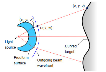
Figure 1 shows a sketch of our design geometry. A point-like light source is located at the origin point, which emits light in the right half space. The curved target surface is described by (x, y, z) and the desired irradiance distribution on it is denoted as L(x, y), where (x, y) are confined in domain Σ. Here, the inner surface of the lens is assumed as spherical. Therefore, our goal is to determine the outer surface (x_f, y_f, z_f), which is generally freeform, to convert the light distribution of the source into the desired irradiance distribution L(x, y). We consider the light source has some arbitrary intensity distributed in the whole semi-sphere. Therefore, Cartesian coordinates are not appropriate here. We prefer using the Stereographic coordinates (u, v) which project the unit sphere X²+Y²+Z²=1 from the south pole (0, 0, -1) onto the z = 0 plane. Generally, (u, v) belong to a unit circular domain which corresponds to the whole semi-sphere where the intensity is defined. However, it is better to implement the calculation with an equi-space rectangular grid. Therefore, we define the coordinates (u, v) on a square domain Ω={(u, v)|-1≤u≤1, -1≤v≤1}, which are used as independent variables for calculation, and transform Ω into a unit circular domain Ωʹ={(uʹ, vʹ)| uʹ²+vʹ²≤1 } using the follow relationships (see Fig. 2):

(uʹ, vʹ) then become the stereographic coordinates and their relationships with (X, Y, Z) can be expressed as:

We will describe the establishment of the outgoing wavefront equation in the following. Assume that the intensity of the light source is denoted as I(uʹ, vʹ), and its stereographically projected irradiance (SPI) on the (uʹ, vʹ) plane can be acquired as¹⁹:

The SPI on the (u, v) plane can be calculated according to energy conservation between the (u, v) and (uʹ, vʹ) planes:

From the differential form of Eq. (4), we can obtain the SPI on the (u, v) plane as:

Energy conservation between source and target can then be expressed as:

where dσ denotes the differential area element of the target surface. Generally, Eq. (6) can be written in the differential form as:

Next, we will link Eq. (7) to the properties of the outgoing wavefront W=(s, t, w). According to Fermat's principle, the gradients of w can be expressed as:

Since s and t are both functions of (u, v), according to the chain rule, we have:

Combining Eqs. (8) and (9), we can describe (x, y) as:

According to the previous IWT method³¹ for a planar target where z is constant, Eq. (10) could explicitly determine x and y as functions of u, v, s, t, w and the first derivatives of s, t and w. We can eliminate the two variables x and y by inserting Eq. (10) into Eq. (7) and thus obtain the final MA equation of w(u, v). However, since we concern a curved target here, z is no longer a constant and becomes a function of x and y: z=z(x, y). Even for a simple case, e.g., z=x²+y², it is very difficult to express x and y explicitly, not to mention the derivation of the final MA equation. Such a fact could also explain why a direct determination of the freeform surface for a curved target is no easy work. However, we can avoid this difficulty artfully by involving z in the following iterative procedure. We consider z as a function of (u, v) and retain it in the right side of Eq. (10). We then insert Eq. (10) into Eq. (7) to obtain a MA equation of w(u, v):

where the coefficients A_i(i=1, 2, 3 and 4) are functions depending on u, v, s, t, w, z, ∂w/∂u, ∂w/∂v, ∂z/∂u, ∂z/∂v and the first and second derivatives of s and t. A nonlinear boundary condition can be specified by applying Eq. (10) for the boundary points.

It is noted that we cannot solve Eq. (11) with the nonlinear boundary condition unless we know s, t and z in advance. That is why we must employ an iterative procedure as shown in Fig. 3. A detailed description of the iterative procedure is provided as follows:

Step 0. We first give initial estimates of z(u, v) and the outgoing wavefront (s(u, v), t(u, v), ŵ(u, v)), where the notation ŵ is used to differentiate from w in the wavefront equation. This could be realized by providing an initial guess of the ray map (x, y) =(x₀(u, v), y₀(u, v)) based on a similar procedure as Step 2 and Step 3.

Step 1. After we have obtained estimates of s(u, v), t(u, v) and z(u, v), we then insert them into Eq. (11) and its boundary condition. Now Eq. (11) has only one unknown w(u, v), which could be solved using a numerical procedure outlined in Ref.³¹. ŵ could be used as an initial estimate of w to start the numerical calculation. A ray map (x, y)=(x(u, v), y(u, v)) can be computed from the solved w through Eq. (10).

Step 2. Based on the ray map obtained in Step 1, we update the z values as: z=z(u, v)=z(x(u, v), y(u, v)).

Step 3. Once we have specified a set of values (x(u, v), y(u, v), z(u, v)) of the target points, we can construct a freeform surface (x_f(u, v), y_f(u, v), z_f(u, v)) using a least squares method¹⁹. An outgoing ray sequence can be obtained by linking (x_f(u, v), y_f(u, v), z_f(u, v)) and (x(u, v), y(u, v), z(u, v)), from which an updated outgoing wavefront (s(u, v), t(u, v), ŵ(u, v)) can be constructed based on least squares.

Step 4. Determine whether the stop criterion is met. A certain iteration number or the ray map deviations from two adjacent iterations could be used as a stop criterion. If the stop criterion is not satisfied, the current values of (s(u, v), t(u, v), ŵ(u, v)) and z(u, v) are inserted into Step 1 again to start a new iteration.

Based on the above iterative procedure, the design complexities could be greatly reduced. Although a sequence of MA equations of the wavefront need to be solved, a multi-scale strategy, which is successfully used in the previous IWT algorithm for planar targets³¹, could be employed to speed up the computation. It is noted that the proposed method is also applicable for more complicated lens geometries, such as plano-freeform, aspherical-freeform or even double freeform lenses.

To verify the proposed method, we first design a freeform lens for producing a flat-top illumination on an undulating surface shown in Fig. 4. This target surface can be expressed as an analytical formula that is modified from Matlab's peaks function:

where (x, y) is confined within the domain Σ={(x, y)| -120≤x≤120, -120≤y≤120} (mm). The target irradiance distribution has the form of a super Gaussian function:

Suppose that the light source located at the origin has a Lambertian intensity distribution, and E(u, v) can be determined using Eqs. (3) and (5). The inner surface of the lens is set as a 12 mm-radius semi-sphere. The refractive index of the lens is set as 1.4932.

The desired computation size is set as 256×256. We implement the computations using the multi-scale strategy run in MATLAB 2019b. The initial computation size is set as 32×32, and a uniform rectangular grid of the target is adopted as the initial ray map. After implementing the procedure shown in Fig. 3 with three iterations, we acquire a 32×32 grid ray map. This ray map is then interpolated into the size of 64×64, which is used to compute the initial estimates of z(u, v) and the outgoing wavefront (x(u, v), y(u, v), ŵ(u, v)) for starting the algorithm on the 64×64 grid. Such a process is repeated until finishing the iteration on the 256×256 grid. In each iteration, we solve the MA equation of the wavefront following the numerical procedure provided in Ref. 31 where a Newton-Krylov solver nsoli.m³⁵ is used. For this example, the source domain involved in computation is set as Ω={(u, v)|-0.94≤u≤0.94, -0.94≤v≤0.94}, and the boundary of (uʹ, vʹ) computed according Eq. (1) is no longer a circle (see Fig. 5(a)). The reason that we employ a smaller source domain is to omit the light rays that are almost parallel to the z=0 plane. These rays may experience total internal reflection, which could result in unreasonable results. Since the light source has Lambertian intensity, only very small amount of energy (~0.21%) is not included in the calculation. Figure 5(b) shows the final ray map. Although the target irradiance distribution is desired as flat-top, we can see from Fig. 5(b) that the ray map is more strongly deformed around the regions of the target which have stronger variations. The z values corresponding to this ray map are specified based on Eq. (12). Following the ray map and its corresponding z values, the final freeform surface (x_f, y_f, z_f) can then be generated based on least squares. The computation ran like ~5 minutes on a Windows 10 desktop PC (Intel Core i7 @ 4.0 GHz with 64 GB RAM). The computed surface data (x_f , y_f , z_f) are given on scattered grid points, which are converted into a 'real' surface using a 3D modeling software, Rhinoceros. The outer freeform surface is then combined with the inner semi-spherical surface to form the final lens model (see Fig. 5(c)). We can see from Fig. 5(c) that the freeform lens is very smooth which could facilitate fabrication. We implement Monte-Carlo simulations using LightTools 8.6 to demonstrate the performance of the designed freeform lens, where 2×10⁶ rays are traced. Figure 6(a) shows the ray tracing results for a point-like light source (size: 10^-3 mm×10^-3 mm). We can see that the simulated irradiance distribution performs very close as the prescribed one.

The second design is more challenging, which aims for generating a letter 'π' and its approximate value '3.14159∙∙∙' in a circular region with the radius of 120 mm on the undulating surface shown in Fig. 4. The irradiance ratio from the uniformly illuminating letter and numbers to the background is set as 4. For this case, we found that the source domain involved in calculation has to be reduced further to obtain reasonable results. Here, we choose the source domain as Ω={(u, v)|-0.8≤u≤0.8, -0.8≤v≤0.8}. The corresponding (uʹ, vʹ) grid is shown in Fig. 6(a). The omitted light source energy still accounts for a very small proportion (~3.1%). After implementing the same numerical procedure as the first design, we acquire the final circular target grid as shown in Fig. 6(b). The computation took like ~4 minutes. From Fig. 6(b), we can clearly see a letter 'π' with very dense grid points, and the regions corresponding to the 'numbers' are also strongly deformed. The final lens model is shown in Fig. 6(c). Compared with the first designed lens shown in Fig. 5(c), the second designed lens is more asymmetric due to its corresponding non-uniform and non-symmetric target irradiance distribution. The simulation results after tracing 1×10⁷ rays are shown in Fig. 6(d). We can observe from Fig. 6(d) a not very sharp irradiance curve along the red dashed line that is across the 'numbers'. Sampling may be a major reason since the 'numbers' are very thin along the red dashed line and there are not enough grid points to render the details at this level. Increasing the computation size may improve the performance. Another reason is that we applied a noise reduction by smoothing with an integral kernel size of three in LightTools.

In the following, we will illustrate the influence of the source size and the distance from the source-lens system to the target surface on the performances of the two designed freeform lenses. Figure 7(a) provides the simulation results for an 1 mm × 1 mm Lambertian source which is commonly used to model an LED source. We can see from Fig. 7(a) that the simulated irradiance distribution still performs well, but there appear to be undulations especially around the biggest bump of the target surface. The irradiance deviation becomes larger when the source size is changed into 2 mm×2 mm, as shown in Fig. 7(b). Overcompensation methods could be used to reduce these irradiance deformations^36-39. Figures 7(c) and 7(d) show the simulation results of the second lens when the source size is changed into 1 mm × 1 mm and 2 mm× 2 mm respectively. We can also observe an irradiance undulation near the biggest bump of the target surface. However, blur effects are more obvious especially in Fig. 7(d). The blur kernels caused by the extended light source is spatially variant partially due to the undulating target surface. Thus, spatially variant deconvolution techniques may make the illumination pattern shaper⁴⁰.

Since we concern irradiance tailoring on a non-planar target, it is necessary to show the effects of the distance from the source-lens system to the target on the simulated irradiance distributions. Figure 8(a) presents the simulated results for the first lens design when the source-lens system is 5 mm closer to the target surface. A hot spot can be clearly observed around the top of the target surface. The hot spot becomes more obvious when the source-lens system is 10 mm closer to the target (see Fig. 8(b)). For the second lens, hot spots also appear when the source-lens system is 5 mm and 10 mm closer to the target surface, as shown in see Figs. 8(c) and 8(d). However, it seems that the distance has little effect on image blur.

A new IWT-based method is proposed for designing freeform lenses that can produce prescribed irradiance distributions on curved targets. The method gradually refines the ray map and its corresponding z-coordinates of the target based on solving a sequence of parameterized wavefront equations. The ray map computed at the i-th iteration is obtained by solving the parameterized wavefront equation which imbeds the scattered z-coordinates of the target at the (i-1)-th iteration, and then the z-coordinates of the target is immediately updated according to the i-th ray map. The high performance of the proposed design method is confirmed by providing two examples of generating a rectangular uniform illumination pattern and an image with circular boundary on an undulating surface from a Lambertian light source. The method was developed under stereographic projection coordinates system, which adopted a special coordinate transformation of the source domain for obtaining reasonable results. In fact, this method may also be applicable for the spherical coordinate system.

In many cases the target cannot be considered as a perfect plane e.g. road surfaces on mountain area, sand tables, surfaces of sculptures and cultural relics. Therefore, we believe that irradiance tailoring on curved targets, which can be generally regarded as 3D surface lighting, can extend the applications of freeform illumination optics.

We are grateful for financial supports from National Key Research and Development Program (Grant No. 2017YFA0701200) and National Science Foundation of China (No. 11704030). The author Z X Feng thanks the valuable discussions with Xu-Jia Wang and Rengmao Wu.

The authors declare no competing financial interests.

References

[1] O Ripoll, V Kettunen, H P Herzig. Review of iterative Fourier-transform algorithms for beam shaping applications. Opt, 43, 2549-2556(2004).
[2] S Keren-Zur, O Avayu, L Michaeli, T Ellenbogen. Nonlinear beam shaping with plasmonic metasurfaces. ACS, 3, 117-123(2016).
[3] G Y Cao, X S Gan, H Lin, B H Jia. An accurate design of graphene oxide ultrathin flat lens based on Rayleigh-Sommerfeld theory. Opto-Electron Adv, 1, 180012(2018).
[4] V D Komissarov, N G Boldyrev. The foundations of calculating specular prismatic fittings. Trudy VEI, 43, 6-61(1941).
[5] J S Schruben. Formulation of a reflector-design problem for a lighting fixture. J Opt Soc Am, 62, 1498-1501(1972).
[6] R M Wu, L Xu, P Liu, Y Q Zhang, Z R Zheng et al. Freeform illumination design: a nonlinear boundary problem for the elliptic Monge-Ampére equation. Opt, 38, 229-231(2013).
[7] H Ries, J Muschaweck. Tailored freeform optical surfaces. J Opt Soc Am A, 19, 590-595(2002).
[8] V Oliker. Mathematical aspects of design of beam shaping surfaces in geometrical optics. In Trends in Nonlinear Analysis, 191-222(2002).
[9] X J Wang. On the design of a reflector antenna Ⅱ. Calc Var Partical Differ Equ, 20, 329-341(2004).
[10] F R Fournier, W J Cassarly, J P Rolland. Fast freeform reflector generation using source-target maps. Opt, 18, 5295-5304(2010).
[11] D Michaelis, P Schreiber, A Bräuer. Cartesian oval representation of freeform optics in illumination systems. Opt, 36, 918-920(2011).
[12] C Canavesi, W J Cassarly, J P Rolland. Target flux estimation by calculating intersections between neighboring conic reflector patches. Opt, 38, 5012-5015(2013).
[13] W A Parkyn. Illumination lenses designed by extrinsic differential geometry. Proc SPIE, 3482, 389-396(1998).
[14] L Wang, K Y Qian, Y Luo. Discontinuous free-form lens design for prescribed irradiance. Appl, 46, 3716-3723(2007).
[15] A Bäuerle, A Bruneton, R Wester, J Stollenwerk, P Loosen. Algorithm for irradiance tailoring using multiple freeform optical surfaces. Opt, 20, 14477-14485(2012).
[16] Y H Yue, K Iwasaki, B Y Chen, Y Dobashi, T Nishita. Poisson-based continuous surface generation for goal-based caustics. ACM Trans Graph, 33, 31(2014).
[17] Y Schwartzburg, R Testuz, A Tagliasacchi, M Pauly. High-contrast computational caustic design. ACM Trans Graph, 33, 74(2014).
[18] D L Ma, Z X Feng, R G Liang. Tailoring freeform illumination optics in a double-pole coordinate system. Appl, 54, 2395-2399(2015).
[19] Z X Feng, B D Froese, R G Liang. Freeform illumination optics construction following an optimal transport map. Appl, 55, 4301-4306(2016).
[20] X L Mao, S B Xu, X R Hu, Y J Xie. Design of a smooth freeform illumination system for a point light source based on polar-type optimal transport mapping. Appl, 56, 6324-6331(2017).
[21] A Bruneton, A Bäuerle, R Wester, J Stollenwerk, P Loosen. Limitations of the ray mapping approach in freeform optics design. Opt, 38, 1945-1947(2013).
[22] R Wester, A Völl, M Berens, J Stollenwerk, P Loosen. Solving the Monge-Ampère equation on triangle-meshes for use in optical freeform design. Proc SPIE, 10693, 1069307(2018).
[23] A Bruneton, A Bäuerle, R Wester, J Stollenwerk, P Loosen. High resolution irradiance tailoring using multiple freeform surfaces. Opt, 21, 10563-10571(2013).
[24] C Bösel, H Gross. Single freeform surface design for prescribed input wavefront and target irradiance. J Opt Soc Am A, 34, 1490-1499(2017).
[25] K Desnijder, P Hanselaer, Y Meuret. Ray mapping method for off-axis and non-paraxial freeform illumination lens design. Opt, 44, 771-774(2019).
[26] L L Doskolovich, D A Bykov, A A Mingazov, E A Bezus. Optimal mass transportation and linear assignment problems in the design of freeform refractive optical elements generating far-field irradiance distributions. Opt, 27, 13083-13097(2019).
[27] D A Bykov, L L Doskolovich, A A Mingazov, E A Bezus, N L Kazanskiy. Linear assignment problem in the design of freeform refractive optical elements generating prescribed irradiance distributions. Opt, 26, 27812-27825(2018).
[28] C R Prins, R Beltman, J H M ten Thije Boonkkamp, W L IJzerman, T W Tukker. A least-squares method for optimal transport using the Monge-Ampère equation. SIAM J Sci Comput, 37, B937-B961(2015).
[29] L B Romijn, J H M ten Thije Boonkkamp, W L IJzerman. Freeform lens design for a point source and far-field target. J Opt Soc Am, 36, 1926-1939(2019).
[30] S L Wei, Z B Zhu, Z C Fan, D L Ma. Least-squares ray mapping method for freeform illumination optics design. Opt, 28, 3811-3822(2020).
[31] Z X Feng, D W Cheng, Y T Wang. Iterative wavefront tailoring to simplify freeform optical design for prescribed irradiance. Opt, 44, 2274-2277(2019).
[32] A Karakhanyan, X J Wang. On the reflector shape design. J Differ Geom, 84, 561-610(2010).
[33] R M Wu, L Yang, Z H Ding, L F Zhao, D D Wang et al. Precise light control in highly tilted geometry by freeform illumination optics. Opt, 44, 2887-2890(2019).
[34] X Sun, L B Kong, M Xu. Uniform illumination for nonplanar surface based on freeform surfaces. IEEE Photonics J, 11, 2200511(2019).
[35] C T Kelley. Solving nonlinear equations with Newton’s method. Society for Industrial and Applied Mathematics(2003).
[36] Y Luo, Z X Feng, Y J Han, H T Li. Design of compact and smooth free-form optical system with uniform illuminance for LED source. Opt, 18, 9055-9063(2010).
[37] Z X Feng, Y Luo, Y J Han. Design of LED freeform optical system for road lighting with high luminance/illuminance ratio. Opt, 18, 22020-22031(2010).
[38] X L Mao, H T Li, Y J Han, Y Luo. Two-step design method for highly compact three-dimensional freeform optical system for LED surface light source. Opt, 22, A1491-A1506(2014).
[39] R Wester, G Müller, A Völl, M Berens, J Stollenwerk et al. Designing optical free-form surfaces for extended sources. Opt, 22, A552-A560(2014).
[40] M Brand, A Aksoylar. Sharp images from freeform optics and extended light sources. Frontiers in Optics(2016).