• High Power Laser Science and Engineering
  • Vol. 11, Issue 2, 02000e28 (2023)
Mikhail Martyanov*, Vladislav Ginzburg, Alexey Balakin, Sergey Skobelev, Dmitry Silin, Anton Kochetkov, Ivan Yakovlev, Alexey Kuzmin, Sergey Mironov, Ilya Shaikin, Sergey Stukachev, Andrey Shaykin, Efim Khazanov, and Alexander Litvak
Author Affiliations
  • Institute of Applied Physics of the Russian Academy of Sciences, Nizhny Novgorod, Russia
  • show less
    DOI: 10.1017/hpl.2023.20 Cite this Article Set citation alerts
    Mikhail Martyanov, Vladislav Ginzburg, Alexey Balakin, Sergey Skobelev, Dmitry Silin, Anton Kochetkov, Ivan Yakovlev, Alexey Kuzmin, Sergey Mironov, Ilya Shaikin, Sergey Stukachev, Andrey Shaykin, Efim Khazanov, Alexander Litvak. Suppressing small-scale self-focusing of high-power femtosecond pulses[J]. High Power Laser Science and Engineering, 2023, 11(2): 02000e28 Copy Citation Text show less

    Abstract

    It was shown experimentally that for a 65-fs 17-J pulse, the effect of filamentation instability, also known as small-scale self-focusing, is much weaker than that predicted by stationary and nonstationary theoretical models for high B-integral values. Although this discrepancy has been left unexplained at the moment, in practice no signs of filamentation may allow a breakthrough in nonlinear pulse post-compression at high laser energy.

    1 Introduction

    The propagation of a high-power laser pulse in a medium with cubic nonlinearity entails a number of physical effects. Many of them are used to control beam parameters: self-phase modulation for white light generation[1], post-compression of femtosecond pulses[24] and pulse amplitude and phase characterization[5,6]; generation of a cross-polarized beam[7]; rotation of a polarization ellipse[8,9]; nonlinear phase shift used for the enhancement of the temporal contrast of a pulse[10,11]; self-focusing of a beam as a whole for mode locking[12]. At the same time, cubic nonlinearity gives rise to destructive effects, which limit the propagation length of high-power laser pulses in optical materials. For example, when a laser pulse is propagating in fibers and capillaries, self-focusing of the beam as a whole limits the pulse power[3], and at second harmonic generation (SHG) self-phase modulation leads to degradation of the phase-matching condition[13,14].

    However, the most significant detrimental effect is small-scale self-focusing (SSSF) occurring in bulk optics, which leads to beam filamentation. This significantly degrades the beam quality and eventually, in most cases, leads to optical breakdown. SSSF is the spatial instability of a plane wave propagating in a medium with cubic nonlinearity – the amplification of transverse spatial perturbations (noise)[15]. The first experimental observation[16] showed a quantitative agreement with the predictions[15]. This stationary theory (i.e., related to the instability of a strong monochromatic plane wave) has been developed in a great variety of works (many of them are referenced in Ref. [17] and, to name a few, the pioneering papers in Refs. [1820]).

    The key conclusion is that the SSSF instability occurs in the $\theta <{\theta}_{{\mathrm{cr}}}$ range, where $\theta =\kappa /{k}_0$ is the angle between the $z$ -axis and the noise transverse wave vector $\kappa$ , ${k}_0=2\pi /\lambda ={\omega}_0/c$ is the longitudinal wave vector of the strong plane wave propagating along the $z$ -axis, ${\omega}_0$ is the optical carrier frequency, $c$ is the speed of light, the critical angle is as follows:

    $$\begin{align}{\theta}_{{\mathrm{cr}}}=2\sqrt{n_0{n}_2{I}_0},\end{align}$$  

    ${n}_{0,2}$ are the linear and nonlinear indexes of refraction correspondingly (such that the total refractive index ${n={n}_0+{n}_2I}$ ) and ${I}_0$ is the plane wave intensity at the input to the nonlinear medium. Hereinafter we use external angles (the angle within the nonlinear medium is $\theta /{n}_0$ ).

    The noise power gain is as follows:

    $$\begin{align*}{K}_{\mathrm{p}}={\left|{E}_{{\mathrm{noise}}}\left(z=L,\overrightarrow{\kappa}\right)\right|}^2/{\left|{E}_{{\mathrm{noise}}}\Big(z=0,\overrightarrow{\kappa}\Big)\right|}^2,\end{align*}$$  

    which is defined as the gain of noise spatial harmonic intensity at spatial frequency $\overrightarrow{\kappa}$ upon propagating the nonlinear plate (NLP) of thickness $L$ . Strictly speaking, ${K}_{\mathrm{p}}$ depends on the noise input phase (see, e.g., Refs. [1921]) and, assuming the random origin of the noise, only the phase-averaged magnitude of ${K}_{\mathrm{p}}$ has practical meaning. The explicit equation for a phase-averaged ${K}_{\mathrm{p}}$ is given in Ref. [4] and reads as follows:

    $$\begin{align}{K}_{\mathrm{p}}\left(\theta \right)=1+\frac{2}{x^2}{\mathrm{sh}}^2(Bx),\end{align}$$  

    where $\gamma =\theta /{\theta}_{{\mathrm{cr}}}$ and $x=2\gamma \sqrt{1-{\gamma}^2}$ . The parameter $B$ is the nonlinear phase shift called the B-integral:

    $$\begin{align}B={k}_0{n}_2{LI}_0,\end{align}$$  

    where $L$ is the length of the nonlinear medium. Note that for $\gamma >1$ , ${K}_{\mathrm{p}}$ is close to unity; for $\gamma =1/\sqrt{2}$ , ${K}_{\mathrm{p}}$ has a maximum value ${K}_{{\mathrm{p}},{\max}}=\mathrm{ch}(2B)$ ; and for small angles $\gamma \ll 1$ , the noise power gain is nearly constant and equal to ${K}_{{\mathrm{p}},0}=1+2{B}^2$ .

    The straightforward extension of this theory (which describes the spatial instability of a plane wave) to high-power optical pulses can be derived assuming time $t$ as a parameter; thus, the B-integral $B(t)={k}_0{n}_2{LI}_0(t)$ and the critical angle ${\theta}_{{\mathrm{cr}}}(t)=2\sqrt{n_0{n}_2{I}_0(t)}$ become time-dependent, where ${I}_0(t)$ is the intensity of the input pulse that spatially stays at the plane wave. In this case, the noise energy gain ${K}_{\mathrm{e}}$ can be derived as a convolution of the power gain ${K}_{\mathrm{p}}$ with the input pulse ${I}_0(t)$ :

    $$\begin{align}{K}_{\mathrm{e}}\left(\theta \right)=\frac{\int {K}_{\mathrm{p}}\left(\theta, t\right)\cdot {I}_0(t) \mathrm{d}t}{\int {I}_0(t) \mathrm{d}t}=1+2\frac{\int {x}^{-2}\mathrm{sh}(Bx){I}_0(t) \mathrm{d}t}{\int {I}_0(t) \mathrm{d}t}.\end{align}$$  

    This approach, which we refer to as stationary, is apparently well justified for nanosecond pulses but rather debatable for much shorter pulses, for example, for the tens of femtoseconds range. As opposed to the stationary approach, the solution of equations that describes the propagation of a short intense laser pulse in a nonlinear dispersive medium hereinafter will be called a nonstationary theory and will be discussed in Section 2.

    Thus, SSSF development is determined, on the one hand, by the noise power and its spatial spectrum at the input to the medium and, on the other hand, by the nonlinearity the measure of which is the B-integral. A large number of experiments with nanosecond pulses showed that the influence of input noise is actually not essential, since the spatial noise cannot be completely eliminated anyway and for the most dangerous angles $\gamma \sim 1/\sqrt{2}$ , the gain ${K}_{\mathrm{p}}$ depends exponentially on $B$ . Therefore, the B-integral is the main parameter that determines the SSSF growth rate, leading to the breakdown of optical elements $B>3$ . This statement, being valid for nanosecond pulses, was erroneously transferred to the femtosecond time scale (see, e.g., Refs. [2225]) and, unfortunately, is continuously repeated, including in recent reviews[2,3]. However, for femtosecond pulses the absence of optical damage and presumably SSSF at $B\gg 3$ was experimentally observed in a number of works[2633]. The reasons for such a significant difference between high-power femtosecond and nanosecond pulses are discussed below and may be divided into two groups: (i) noise power reduction at the input to the nonlinear medium and (ii) noise gain ${K}_{\mathrm{p}}$ and ${K}_{\mathrm{e}}$ reduction.

    1.1 The reduction of noise power at the input to the nonlinear medium

    For nanosecond lasers, a typical beam intensity is several $\mathrm{GW}/{\mathrm{cm}}^2$ , which gives ${\theta}_{{\mathrm{cr}}}$ of about 1 mrad; for femtosecond lasers, the typical intensity is several $\mathrm{TW}/{\mathrm{cm}}^2$ and the angle ${\theta}_{{\mathrm{cr}}}$ is already tens of mrad. Such a substantial increase in ${\theta}_{{\mathrm{cr}}}$ leads to a decrease in the spectral density in the most ‘hazardous’ region $\gamma \sim 1/\sqrt{2}$ due to three effects.

    The first of them is spatial self-filtering of the beam during propagation in free space[32]. If the nonlinear medium is rather far away from the noise source (NS; which is in most cases any optical surface touched by the beam), then the most ‘hazardous’ noise transverse spatial frequency ${\mid {\overrightarrow{\kappa}}_{{\mathrm{cr}}}\mid ={k}_0{\theta}_{{\mathrm{cr}}}}$ simply walks-off from the beam aperture; the larger the ${\theta}_{{\mathrm{cr}}}$ , the smaller the distances required for spatial self-filtering. This effect was experimentally confirmed qualitatively[26,32] and quantitatively[34]. Second, for short pulses, free space is also a temporal filter[35], separating the noise pulse from the main pulse in time rather than in space. Since high spatial frequency noise propagates at an angle to the $z$ -axis, it lags behind the main pulse. As the delay becomes comparable with the pulse duration, the maximum intensity of the main pulse ‘meets’ the leading edge of the noise, which is equivalent to a reduction of input noise power. With the increase of the delay, the reduction may be exponentially small. Third, the noise spatial spectral density evidently decreases as $\theta$ increases. The particular model noise spectra were simulated in Ref. [36]. The results showed that this effect can significantly reduce SSSF; however, this strongly depends on the spectral density decay law, which requires a special experimental study.

    1.2 Substantial reduction of noise gain for short pulses

    The spatiotemporal instability of a plane wave in the approximation of a slowly varying amplitude was investigated in Ref. [37] and an expression for the instability increment taking into account higher-order dispersions, spatiotemporal focusing (the nonstationary diffraction term) and self-steepening was obtained in Ref. [38]. Analytical expressions for the noise power gain similar to Equation (2) cannot be obtained. In Refs. [39,40], the development of SSSF was studied without the approximation of slowly varying amplitude. It was shown numerically that, in the case of anomalous dispersion, SSSF does not develop for laser pulses with a duration of less than 10 field periods. Experimental confirmation of this effect has not been demonstrated. Moreover, with normal dispersion, this effect has not been studied either theoretically or in simulation.

    In Section 2 of this work we perform a detailed analysis of noise gain at nonstationary nonlinear interaction and determine the parameters at which SSSF is suppressed. Results of the measurements of spatial noise gain and their comparison with the stationary theory (Equation (4)) and numerical simulation of the nonstationary problem considered in Section 2 are presented in Section 3.

    2 Numerical simulation

    The numerical simulation of SSSF was performed using two approaches. The first one is based on the slowly varying amplitude approximation that gives a modified nonlinear Schrödinger equation (NSE) for a complex field amplitude $\overrightarrow{U}\left(t,z,\overrightarrow{r}\right)$ [38,41]. It is convenient to write the NSE using normalized time $t$ , $z$ and $r$ coordinates and normalized scalar field $\Psi$ (assuming linear polarization) as follows:

    $$\begin{align}\xi =\frac{z}{L},\kern-1pt\quad \eta =\frac{t-z/u}{\tau_0},\kern-1pt\quad \overrightarrow{\rho}=\overrightarrow{r}\sqrt{\frac{k_0{n}_0}{L}},\kern-1pt\quad \Psi =\frac{U}{\sqrt{I_0}},\end{align}$$  

    where $u={\left(\partial k/\partial \omega \right)}^{-1}$ is the group velocity at frequency ${\omega}_0$ , ${I}_0$ is the maximum of the input pulse intensity (the field unit is the square root of intensity) and ${\tau}_0$ is the duration of the input pulse. With Equation (5) taken into account, the NSE has the following form:

    $$\begin{align}\begin{array}{l}\left(\frac{\partial }{\partial \xi }-\frac{i}{2}D\frac{\partial^2}{\partial {\eta}^2}-\frac{i}{2}\left(1-\frac{i}{2\pi N}\frac{\partial }{\partial \eta}\right){\varDelta}_{\overrightarrow{\rho}}\right)\Psi =\\ {}\kern7em - iB\left(1+\frac{i}{2\pi N}\frac{\partial }{\partial \eta}\right){\left|\Psi \right|}^2\Psi, \end{array}\end{align}$$  

    where

    $$\begin{align}N={\tau}_0/T,\end{align}$$  

    $$\begin{align}D={k}_2L/{\tau}_0^2,\end{align}$$  

    ${k}_2={\left.\frac{\partial^2k}{\partial {\omega}^2}\right|}_{\omega_0}$ is the group velocity dispersion and $T=\lambda /c=2\pi /{\omega}_0$ is the optical field period.

    The second approach proposed in Refs. [4244] is based on the unidirectional wave equation (UWE) for a complete oscillating optical complex field $\overrightarrow{E}\left(t,z,\overrightarrow{r}\right)=\overrightarrow{U}\left(t,z,\overrightarrow{r}\right){e}^{i{\omega}_0t}$ with the assumption of the particular optical dispersion, which is explicitly written for dielectric permittivity as $\varepsilon ={\varepsilon}_0+{\alpha \omega}^2$ . Note that, if this particular empirical dispersion law is supposed to be used in the optical band for reasonable optical materials, then the parameters ${\varepsilon}_0$ and $\alpha$ have to be chosen accordingly to mimic the physical dispersion. It turns out that for realistic materials, ${\varepsilon}_0\gg {\alpha \omega}_0^2$ and the refractive index in the optical band is $n\approx {n}_0+{\alpha \omega}^2/2$ , where ${n}_0=\sqrt{\varepsilon_0}\approx c/u$ and the dispersion coefficients are ${k}_2\approx 3\alpha {k}_0/{n}_0$ and ${k}_3\approx 3\alpha /{cn}_0$ . The equation for the normalized optical complex scalar field $\Psi =E/\sqrt{I_0}$ (assuming linear polarization) in the UWE approximation with the same coordinate normalization (Equation (5)) can be written as follows:

    $$\begin{align}\left(\frac{\partial^2}{\partial \xi \partial \eta }-\frac{D}{12\pi N}\frac{\partial^4}{\partial {\eta}^4}-\pi N{\varDelta}_{\overrightarrow{\rho}}\right)\Psi =\frac{B}{2\pi N}\frac{\partial^2}{\partial {\eta}^2}{\left|\Psi \right|}^2\Psi .\end{align}$$  

    Third- and higher-order dispersions as well as the third harmonic generation are already neglected in the NSE (Equation (6)). The UWE (Equation (9)) intrinsically contains second and third dispersion orders. Using the same definition (Equation (8)) one can obtain $D=3\alpha {k}_0L/{n}_0{\tau}_0^2$ . As for the third harmonic generation, it was also neglected in the UWE (Equation (9)).

    From Equations (6) and (9) it is clear that the nonstationary problem depends, besides the B-integral (Equation (3)), on two dimensionless parameters, $N$ and $D$ . Note that the $D/B$ ratio is equal to the ratio of the nonlinear length ${{L}_{{\mathrm{nl}}}=1/\left({k}_0{n}_2{I}_0\right)}$ to the dispersion length ${L}_{\mathrm{d}}={\tau}_0^2/{k}_2$ .

    Instead of $D$ , another parameter $C$ can be introduced, which (in contrast to $D$ ) is convenient in that it depends neither on the input pulse duration nor on the nonlinear medium length $L$ :

    $$\begin{align}C=2{\pi}^2\frac{DN^2}{B}=\frac{k_0{c}^2{k}_2}{2{n}_2{I}_0}.\end{align}$$  

    Parameter $C$ appears naturally in the wave equations (Equations (6) and (9)) if the longitudinal coordinate $z$ were normalized to $L/B$ , that is, $\tilde{\xi}= Bz/L$ , and time $t$ were normalized to the optical period $T$ .

    Both Equations (6) and (9) were solved numerically for identical parameters and boundary conditions. An intense pulse with uniform spatial distribution combined with weak spatial noise with the same temporal shape was fed to the nonlinear medium input ( $z=0$ ), and the noise energy gain was calculated:

    $$\begin{align}K\left(\theta \right)=\frac{\iint_0{\left|{E}_{{\mathrm{noise}}, {\mathrm{out}}}\left(t,\overrightarrow{\kappa}\right)\right|}^2 \mathrm{d}t\mathrm{d}\phi}{\iint_0{\left|{E}_{{\mathrm{noise}}, {\mathrm{in}}}\left(t,\overrightarrow{\kappa}\right)\right|}^2 \mathrm{d}t\mathrm{d}\phi},\end{align}$$  

    where $\phi$ is the polar angle in $\overrightarrow{\kappa}$ -space. The noise input phase was a random function uniformly distributed in the interval from 0 to 2 $\pi$ . The integration over the polar angle $\phi$ in Equation (11) replaces the averaging over multiple realizations of randomly distributed input noise phase.

    We restricted the consideration to the linear regime, when the noise growth had no back-action on the strong pulse. For this, the noise amplitude was chosen so small that even at the output of the nonlinear medium it stayed much smaller than the amplitude of the strong pulse. The field of the strong wave at the input ${E}_{{\mathrm{in}}}\left(t,z=0\right)$ did not depend on the transverse coordinates and in time it was a Gaussian pulse with duration ${\tau}_0$  :  ${E}_{{\mathrm{in}}}\left(t,z=0\right)={E}_0{e}^{-{\left(t/{\tau}_0\right)}^2/2}$ . The noise had the same temporal shape, and its spatial spectrum was much wider than the instability range. The shape of the spatial spectrum was of no importance for calculating $K$ .

    The results of numerical simulation showed that Equations (6) and (9) give similar results. The solid curves for $K\left(\gamma \right)$ obtained using Equation (6) are plotted in Figure 1. For ${N=50}$ , the simulation results agree very well with Equation (4) – the dashed and solid curves overlap in all four Figures 1(a)–1(d). For shorter pulses, the magnitudes of $K$ are significantly smaller, and the $K$ maximum shifts from $\gamma =1/\sqrt{2}$ towards smaller $\gamma$ . This has a simple physical explanation. Due to normal dispersion, the strong pulse is subjected to stretching as it propagates through a nonlinear medium, and thus its peak intensity decreases and as a result the overall nonlinear phase shift at the medium output is less than the B-integral determined by Equation (3). The effective B-integral can be defined as follows:

    $$\begin{align}{B}_{{\mathrm{eff}}}={k}_0{n}_2\underset{t}{\max }{\int}_0^LI\left(t,z\right) \mathrm{d}z,\end{align}$$  

    Gain as a function of for (a), (c) and (b), (d); (a), (b) and (c), (d); for (black curves), (green curves), (red curves) and (blue curves). The solid curves show the results of numerical simulation, while the dashed curves are plotted by Equation (4), with replaced by .

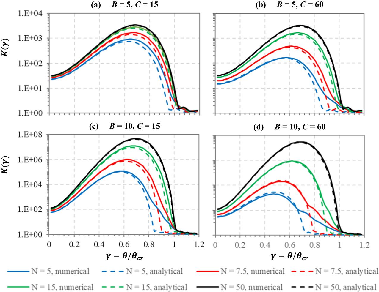
    Figure 1.Gain as a function of for (a), (c) and (b), (d); (a), (b) and (c), (d); for (black curves), (green curves), (red curves) and (blue curves). The solid curves show the results of numerical simulation, while the dashed curves are plotted by Equation (4), with replaced by .

    where the intensity $I\left(t,z\right)$ is the solution of Equation (6) or (9) that describes the evolution of a strong pulse in a dispersive nonlinear medium. If ${B}_{{\mathrm{eff}}}$ is substituted for $B$ in Equation (4), the result for the noise becomes quite close to the solution of Equation (6) (comparing the solid and dashed curves in Figure 1). In particular, both the maximum values of $K$ and the values of $\gamma$ at which $K$ has a maximum agree well. There is a significant difference only at the angles close to $\gamma \sim 1$ . This difference is mainly related to the definitions of ${\theta}_{{\mathrm{cr}}}$ and $B$ (Equations (1) and (2)) that make the critical angle proportional to the square root of $B$ . Therefore, the replacement of $B$ by ${B}_{{\mathrm{eff}}} makes the critical angle by factor $\sqrt{B_{{\mathrm{eff}}}/B}<1$ lower. This, in turn, makes the stationary analytic dashed curves in Figure 1 bump into the horizontal axis at a value lower than $\gamma =1$ . At the same time, in the accurate numerical simulation (solid curves in Figure 1) there is some noise gain even at the angles close to ${\gamma =1}$ , which occurs in the beginning of the pulse propagation until the pulse is not yet stretched and the peak intensity is still high. Thus, the suppression of SSSF for shorter pulses (smaller $N$ ) can be explained by the pulse stretching due to normal dispersion, which effectively decreases the value of the $B$ -integral down to ${B}_{{\mathrm{eff}}}$ .

    Using the results obtained in Ref. [45], it can be easily shown that the durations of the input and output pulses practically do not differ if $BD\ll 0.5$ . Otherwise, the pulse is stretched and $K$ decreases. The decrease in peak intensity due to stretching during pulse propagation also explains the shift of the $K$ maximum towards smaller $\gamma$ , as ${\theta}_{{\mathrm{cr}}}$ is proportional to the square root of the intensity (Equation (1)) and, therefore, decreases during propagation.

    3 Experimental results and discussion

    The experimental layout is shown in Figure 2. A beam of the laser PEARL (PEtawatt pARametric Laser[46]) with central wavelength 910 nm, pulse energy up to 17 J, full width at half maximum (FWHM) pulse duration 65 fs (N = 13) and diameter 18 cm passed through an orifice with a diameter of 10 cm located in vacuum at a distance of 8 m from the last compressor grating. The purpose of the orifice was to trim out the lateral wings of the beam to make the residual central part more like a flat-top for better interpretation of the results. The intensity averaged across the nearly flat-top beam was 0.8 $\mathrm{TW}/{\mathrm{cm}}^2$ . Next, the beam propagated through a thin glass plate, which introduced a spatial NS and an NLP. The distance between the orifice and the NS was 2 cm and that between the NS and NLP 3 cm; thus, the diffraction on the orifice’s hard edge was insignificant within the NLP. Glass (BK7) with a thickness of 7 mm or a potassium dihydrogen phosphate (KDP) crystal with a thickness of 4 mm was used as an NLP. The values of $B$ and $C$ in these two cases were $B=14$ and 10, $C=37$ and 9.6, respectively. The 0.5-mm thick randomly scratched glass plate was used as an NS and was placed just in front of the NLP. The distance between the NS and the NLP was set small enough (3 cm) to exclude spatial[32] and temporal[35] self-filtering. Downstream of the NLP, the beam upon reflection from two wedges was attenuated by about a factor of 1000 and escaped from the vacuum chamber. The B-integral in the vacuum window did not exceed 0.05. In the focal plane of the lens ( $F=73$ cm), there was a mirror with a pinhole (PHM) 2.5 mm in diameter through which the core of the laser beam associated with the strong pulse and large transverse size easily passed. The halo consisting of the spatial noise was reflected by the PHM. The PHM plane was image relayed onto the charge-coupled device (CCD) camera. Note that the wedges, the vacuum viewport and the lens had the apertures large enough to transfer the spatial frequencies up to ${\theta <5.5}$ mrad without significant distortion. Therefore, the CCD camera captured the time-integrated noise spatial spectrum in the $2\ \mathrm{mrad}<\theta <5.5\ \mathrm{mrad}$ range, all of which is in the $\theta \ll {\theta}_{{\mathrm{cr}}}$ range ( ${\theta}_{{\mathrm{cr}}}\approx 40$ mrad in our case).

    Experimental layout. NS – noise source (randomly scratched 0.5 mm thick glass plate), NLP – nonlinear plate (BK7 glass or KDP), PHM – mirror with a pinhole.

    Figure 2.Experimental layout. NS – noise source (randomly scratched 0.5 mm thick glass plate), NLP – nonlinear plate (BK7 glass or KDP), PHM – mirror with a pinhole.

    First of all, the NS scratch density was chosen such that most of the noise was introduced by the NS, whereas the noise from the other optical elements located both upstream and downstream of the NLP could be neglected (comparing the black and green curves in Figure 3(a)). These measurements were made in a linear regime with $B\ll 1$ . The blue and red curves in Figure 3(a) show the noise spectra for glass and KDP crystal, respectively. The ratio of the nonlinear and linear spectra, that is, noise gain $K\left(\theta \right)$ , is shown by solid curves in Figure 3(b). Note that these curves have been plotted assuming that all the noise was generated upstream of the NLP on the NS, which is not entirely true. An upper estimate can be made assuming that all the noise without the NS (black curve in Figure 3(a)) was not amplified, since it was ‘born’ downstream of the NLP. The dashed curves in Figure 3(b) correspond to $K\left(\theta \right)$ calculated in accordance with this assumption.

    Experimental noise spectra (a) and noise gain (b).

    Figure 3.Experimental noise spectra (a) and noise gain (b).

    A small modulation of the function $K\left(\theta \right)$ could be associated with the fact that the NS was at some particular distance from the NLP (see Ref. [21] for detail). From Figure 3(b) it is clear that the values of $K$ for glass and KDP crystal slightly differ from each other, but in general we can conclude that $K\approx 2$ , and the upper estimate is $K<5$ in both cases. The quasi-stationary theory (Equation (4)) at $\theta \ll {\theta}_{{\mathrm{cr}}}$ for a Gaussian pulse gives ${K}_{\mathrm{e}}=1+2{B}^2/\sqrt{3}$ , that is, ${K}_{\mathrm{e}}=116$ for $B=10$ (KDP) and ${K}_{\mathrm{e}}=227$ for $B=14$ (glass). The results of the simulation (Equation (6)) yield $K=106$ and 112 for KDP and glass, respectively, which also greatly exceed the measured values.

    Thus, the experimental results demonstrate significant suppression of SSSF at $\theta \ll {\theta}_{{\mathrm{cr}}}$ , which cannot be explained by the existing theoretical concepts. Possible reasons for this discrepancy could be the following. First, Equations (6) and (9) do not take into account the finite temporal response of Kerr nonlinearity (it was assumed to be inertia-free, i.e., instant), which can lead to the generation of Raman-shifted waves. Second, in simulation the temporal shape of the noise at the input to the nonlinear medium coincided with that of the strong pulse, which may not exactly correspond to the experimental conditions. Third, in the simulation both the amplitude and the phase of the strong beam were assumed to be ideally uniform in space (plane wave), while in the experiment the beam had a large-scale structure. Fourth, the plane wave depletion was not considered in the simulation, so the spatial noise intensity was kept low even at the output of the NLP. In reality, this assumption may be easily violated. The well-known example is the so-called beam hot spots, which may be considered as the ultimate stage of SSSF when the noise absorbs a substantial fraction of the main beam energy. Clarification of the exact reason for the discrepancy between the theoretical and experimental data is the subject of our further research.

    4 Conclusion

    The detailed numerical simulation of the propagation of femtosecond laser pulses in a medium with Kerr nonlinearity showed that, in the case of normal dispersion (in contrast to anomalous dispersion[39,40]), SSSF is not suppressed. Even for short laser pulses, noise gain is well described by the stationary theory (Equations (2) and (4)) if the B-integral (Equation (3)) is replaced by ${B}_{{\mathrm{eff}}}$ (Equation (12)). Nevertheless, the considerable reduction of noise gain, which may be considered as the suppression of SSSF, was observed experimentally. Direct measurements of the noise gain showed its significant decrease in comparison with both the quasi-stationary theory and numerical simulations. The explanation for this discrepancy needs further study, but in practice no signs of filamentation enables successful implementation of nonlinear pulse post-compression at high laser energy and high B-integral values, resulting in a higher compression ratio and peak power.

    References

    [1] A. Dubietis, G. Tamošauskas, R. Šuminas, V. Jukna, A. Couairon. Lith. J. Phys., 57(2017).

    [2] M. Hanna, F. Guichard, N. Daher, Q. Bournet, X. Délen, P. Georges. Laser Photon. Rev., 15, 2100220(2021).

    [3] T. Nagy, P. Simon, L. Veisz. Adv. Phys. X, 6, 1845795(2020).

    [4] E. A. Khazanov, S. Y. Mironov, G. Mourou. Uspekhi Fizicheskih Nauk, 189, 1173(2019).

    [5] E. A. Anashkina, V. N. Ginzburg, A. A. Kochetkov, I. V. Yakovlev, A. V. Kim, E. A. Khazanov. Sci. Rep., 6, 33749(2016).

    [6] A. V. Andrianov, A. V. Kim, E. A. Khazanov. Quantum Electron., 47, 236(2017).

    [7] A. Jullien, O. Albert, F. Burgy, G. Hamoniaux, J.-P. Rousseau, J.-P. Chambaret, F. Augé-Rochereau, G. Chériaux, J. Etchepare, N. Minkovski, S. M. Saltiel. Opt. Lett., 30, 920(2005).

    [8] K. Sala, M. C. Richardson. J. Appl. Phys., 49, 2268(1978).

    [9] N. G. Khodakovskiy, M. P. Kalashnikov, V. Pajer, A. Blumenstein, P. Simon, M. M. Toktamis, M. Lozano, B. Mercier, Z. Cheng, T. Nagy, R. Lopez-Martens. Laser Phys. Lett., 16, 095001(2019).

    [10] E. Khazanov. Opt. Express, 29, 17277(2021).

    [11] D. Silin, E. Khazanov. Opt. Express, 30, 4930(2022).

    [12] D. E. Spence, P. N. Kean, W. Sibbett. Opt. Lett., 16, 42(1991).

    [13] T. Ditmire, A. M. Rubenchik, D. Eimerl, M. D. Perry. J. Opt. Soc. Am. B, 13, 649(1996).

    [14] S. Y. Mironov, V. N. Ginzburg, V. V. Lozhkarev, G. A. Luchinin, A. V. Kirsanov, I. V. Yakovlev, E. A. Khazanov, A. A. Shaykin. Quantum Electron., 41, 963(2011).

    [15] V. I. Bespalov, V. I. Talanov. JETP Lett., 3, 471(1966).

    [16] Y. S. Chilingarian. JETP, 55, 1589(1968).

    [17] A. J. CampilloSelf-focusing: Past and Present, 157(2009).

    [18] B. Suydam. IEEE J. Quantum Electron., 10, 837(1974).

    [19] C. Elliott, B. Suydam. IEEE J. Quantum Electron., 11, 863(1975).

    [20] N. N. Rosanov, V. A. Smirnov. Soviet J. Quantum Electron., 10, 232(1980).

    [21] A. K. Potemkin, E. A. Khazanov, M. A. Martyanov, M. S. Kochetkova. IEEE J. Quantum Electron., 45, 336(2009).

    [22] G. Mourou, G. Cheriaux, C. Radier. , , and , “Device for generating a short duration laser pulse.” Patent US20110299152A1 (2014-08-05)..

    [23] S. N. Vlasov, E. V. Koposova, V. E. Yashin. Quantum Electron., 42, 989(2012).

    [24] A. A. Mak, V. E. Yashin. Opt. Spectrosc., 70, 1(1991).

    [25] A. A. Andreev, A. A. Mak, V. E. Yashin. Quantum Electron., 27, 95(1997).

    [26] S. Mironov, V. Lozhkarev, G. Luchinin, A. Shaykin, E. Khazanov. Appl. Phys. B, 113, 147(2013).

    [27] A. Shaykin, V. Ginzburg, I. Yakovlev, A. Kochetkov, A. Kuzmin, S. Mironov, I. Shaikin, S. Stukachev, V. Lozhkarev, A. Prokhorov, E. Khazanov. High Power Laser Sci. Eng, 9, e54(2021).

    [28] V. Ginzburg, I. Yakovlev, A. Kochetkov, A. Kuzmin, S. Mironov, I. Shaikin, A. Shaykin, E. Khazanov. Opt. Express, 29, 28297(2021).

    [29] V. Ginzburg, I. Yakovlev, A. Zuev, A. Korobeynikova, A. Kochetkov, A. Kuzmin, S. Mironov, A. Shaykin, I. Shaikin, E. Khazanov, G. Mourou. Phys. Rev. A, 101, 013829(2020).

    [30] V. N. Ginzburg, I. V. Yakovlev, A. S. Zuev, A. P. Korobeynikova, A. A. Kochetkov, A. A. Kuzmin, S. Yu. Mironov, A. A. Shaykin, I. A. Shaikin, E. A. Khazanov. Quantum Electron., 50, 331(2020).

    [31] P. Lassonde, S. Mironov, S. Fourmaux, S. Payeur, E. Khazanov, A. Sergeev, J.-C. Kieffer, G. Mourou. Laser Phys. Lett., 13, 075401(2016).

    [32] S. Y. Mironov, V. V. Lozhkarev, V. N. Ginzburg, I. V. Yakovlev, G. Luchinin, A. Shaykin, E. A. Khazanov, A. Babin, E. Novikov, S. Fadeev, A. M. Sergeev, G. A. Mourou. IEEE J. Select. Top. Quantum Electron., 18, 7(2012).

    [33] J. I. Kim, Y. G. Kim, J. M. Yang, J. W. Yoon, J. H. Sung, S. K. Lee, C. H. Nam. Opt. Express, 30, 8734(2022).

    [34] V. N. Ginzburg, A. A. Kochetkov, A. K. Potemkin, E. A. Khazanov. Quantum Electron., 48, 325(2018).

    [35] E. A. Khazanov. Quantum Electron., 52, 208(2022).

    [36] V. N. Ginzburg, A. A. Kochetkov, S. Y. Mironov, A. K. Poteomkin, D. E. Silin, E. A. Khazanov. Izv. VUZov. Radiofizika, 62, 953(2019).

    [37] A. G. Litvak, V. I. Talanov. Izv. VUZov. Radiofizika, 10, 539(1967).

    [38] L. Bergé, S. Mauger, S. Skupin. Phys. Rev. A, 81, 013817(2010).

    [39] A. A. Balakin, A. V. Kim, A. G. Litvak, V. A. Mironov, S. A. Skobelev. Phys. Rev. A, 94, 043812(2016).

    [40] A. A. Balakin, A. G. Litvak, V. A. Mironov, S. A. Skobelev. J. Opt., 19, 095503(2017).

    [41] T. Brabec, F. Krausz. Phys. Rev. Lett., 78, 3282(1997).

    [42] V. G. Bespalov, S. A. Kozlov, Y. A. Shpolyanskiy, I. A. Walmsley. Phys. Rev. A, 66, 013811(2002).

    [43] A. A. Balakin, A. G. Litvak, V. A. Mironov, S. A. Skobelev. Phys. Rev. A, 78, 061803(2008).

    [44] A. A. Balakin, A. G. Litvak, V. A. Mironov, S. A. Skobelev. Phys. Rev. A, 80, 063807(2009).

    [45] A. Zheltikov. Opt. Express, 26, 17571(2018).

    [46] V. V. Lozhkarev, G. I. Freidman, V. N. Ginzburg, E. V. Katin, E. A. Khazanov, A. V. Kirsanov, G. A. Luchinin, A. N. Mal’shakov, M. A. Martyanov, O. V. Palashov, A. K. Poteomkin, A. M. Sergeev, A. A. Shaykin, I. V. Yakovlev. Laser Phys. Lett., 4, 421(2007).

    Mikhail Martyanov, Vladislav Ginzburg, Alexey Balakin, Sergey Skobelev, Dmitry Silin, Anton Kochetkov, Ivan Yakovlev, Alexey Kuzmin, Sergey Mironov, Ilya Shaikin, Sergey Stukachev, Andrey Shaykin, Efim Khazanov, Alexander Litvak. Suppressing small-scale self-focusing of high-power femtosecond pulses[J]. High Power Laser Science and Engineering, 2023, 11(2): 02000e28
    Download Citation