A. Marcu, M. Stafe, M. Barbuta, R. Ungureanu, M. Serbanescu, B. Calin, N. Puscas. Photon energy transfer on titanium targets for laser thrusters[J]. High Power Laser Science and Engineering, 2022, 10(5): 05000e27
Copy Citation Text
Using two infrared pulsed lasers systems, a picosecond solid-state Nd:YAG laser with tuneable repetition rate (400 kHz–1 MHz) working in the burst mode of a multi-pulse train and a femtosecond Ti:sapphire laser amplifier with tuneable pulse duration in the range of tens of femtoseconds up to tens of picoseconds, working in single-shot mode (TEWALASS facility from CETAL-NILPRP), we have investigated the optimal laser parameters for kinetic energy transfer to a titanium target for laser-thrust applications. In the single-pulse regime, we controlled the power density by changing both the duration and pulse energy. In the multi-pulse regime, the train’s number of pulses (burst length) and the pulse energy variation were investigated. Heat propagation and photon reflection-based models were used to simulate the obtained experimental results. In the single-pulse regime, optimal kinetic energy transfer was obtained for power densities of about 500 times the ablation threshold corresponding to the specific laser pulse duration. In multi-pulse regimes, the optimal number of pulses per train increases with the train frequency and decreases with the pulse power density. An ideal energy transfer efficiency resulting from our experiments and simulations is close to about 0.0015%.
Laser–matter interaction is a rather complex process representing a broad research domain with numerous scientific and technology applications in various domains of activities, from engineering and nanotechnology to medicine and astronomy[1–7]. The photon is known as a mass-less particle in the quantum physics approach, but it is still able to transfer impulse and respectively kinetic energy to macroscopic targets
$\left({E}_\mathrm{p}={h}_{\mathrm{Planck}}\cdot \nu \right)$
. Because the Planck constant
${h}_\mathrm{Planck}$
has a very small value of about
${10}^{-34}$
m2 · kg/s, transferred energy usually has a neglectable value at the macroscopic scale, but since the total transferred energy depends on the total number of photons and the photon-associated frequency, there are cases, and consequently applications, where this energy is no longer neglectable. Transferred impulse and respectively kinetic energy while irradiating started to be experimentally measured from the beginning of the 20th century based on the Maxwell theoretical model[8] and were later studied for laser-thrust possible applications[9–12]. More recent applications based on ultrashort and ultra-intense pulse light radiation-induced pressure were investigated from the point of view of induced shock waves inside the solid target[13,14] and even particle acceleration, such as ions[15], to relativistic energies. According to the theory, if the laser peak power density (intensity) exceeds values of
${10}^{24}$
W/cm2 on a target thicker than several atomic layers, after being fully ionized it will act as a plasma mirror that will reflect the incident pulse, taking a significant amount of its impulse[16]. It is known that kinetic energy transfer efficiency depends on several parameters, such as the laser wavelength and target material, but for a given target material and a particular laser beam it mostly depends on the beam power density on the target[17]. However, in a pulsed laser system, the power density can be changed by controlling three main parameters: the pulse energy, beam size or pulse duration. Since for real applications changing the beam size (respectively changing the focus position while following a moving target) is not always a practical solution, studies usually address the other two ways: controlling pulse energy and respectively pulse duration. While the existing experimental studies on light pulse kinetic energy transfer to targets are performed on rather limited power range intervals – usually obtained by varying only the pulse energy – corroborated studies on wider ranges mostly rely on combined individual studies performed with rather different laser wavelength, pulse duration and target material[12]. In terms of pulse duration, previous studies have shown that for long laser pulses (e.g., ns or longer), the dissipation of the absorbed energy in the bulk material and possibly material removal take place during the laser pulse duration[18]. For pulses shorter than the characteristic relaxation time (e.g., below a few ps) during the laser–matter interaction process, the photon energy will be transferred to the electrons and they will further transfer it to the target atoms as electron-to-ion energy transfer. All of these processes typically occur of the order of several picoseconds after laser absorption. Hence, for short laser pulses, heat diffusion is confined during the interaction of the laser beam with material, and the shock-like energy transfer leads to ablation. Thus, there should be significant differences between controlling the power density by energy and by pulse duration. In the present work, we start with a systematic study in single-shot mode on the correlation between the laser pulse power density and the efficiency of kinetic energy transfer for a given target (titanium in our case) with fixed geometry using an infrared (IR) pulsed laser beam (Ti:sapphire chirped pulse amplification (CPA) laser amplifier at the TEWALAS facility part of CETAL INFLPR). For this purpose, we varied the pulse duration while maintaining the pulse energy, and vice versa. Because in a propulsion application, more pulses (train of pulses) will be more likely needed, we have further investigated the influence of the number of pulses, repetition rate and energy per pulse over the kinetic energy transfer within the range of our experimental tools of 1 MHz repetition rate. For a deeper understanding of the obtained data and processes, the experimental results were compared with computer simulations of photo-thermal-induced effect models[18–22] with similar (or comparable) laser–target interaction parameters.
2 Theoretical modelling and preliminary calculations
The presence of a gas next to the irradiated surface (due to the low vacuum and multi-pulse regime employed in our experiments) leads to very important thermal evaporation after the pulse as compared to the non-thermal ablation mechanism, which is valid for ultrashort laser pulses (smaller than picoseconds) in vacuum[23]. Thus, we can consider that thermal ablation is the main ablation mechanism during and after a laser pulse with duration
$\tau$
of the order of ps or longer, at laser intensities above the ablation threshold.
The ablation is initiated by the absorption of the laser energy by the free electrons via the inverse Bremsstrahlung process, followed by rapid (picosecond scale) relaxation of the energy via electron–electron and electron–phonon collisions[23]. Thereby, at the long timescale of 100
$\tau$
employed in this study, the two sub-systems (i.e., electrons and phonons) can be considered in thermal equilibrium and the temperature distribution in the target can be described by a single heat equation, regardless of the pulse duration.
Sign up for High Power Laser Science and Engineering TOC. Get the latest issue of High Power Laser Science and Engineering delivered right to you!Sign up now
The thermal penetration depth is
${l}_\mathrm{T}=2\sqrt{D\tau}$
, where
$D$
is the thermal diffusivity of the target and
$\tau$
is the laser pulse duration. Accounting for the pulse duration involved in this study (mostly ps regimes), the thermal penetration depth is in the range of 5 μm–5 nm, which is very small as compared to the laser beam diameter
$d$
= 3 mm on the target surface. Thus, the temperature distribution in the axial
$z$
-direction can be determined from the 1D heat equation [18–21,24]:
Here,
$\rho$
,
${c}_\mathrm{p}$
and
$k$
denote the mass density, the specific heat and the thermal conductivity of titanium, respectively, which are taken as constant parameters. The source term of the heat equation describes the volumetric laser energy input near the irradiated surface:
where
${l}_\mathrm{p}$
and
${\alpha}_\mathrm{p}$
are the total length and the absorption coefficient of the plasma plume, respectively, and the surface reflectivity
$R$
= 0.61 and the optical absorption coefficient of the target,
$\alpha =2.36\times{10}^7$
cm–1, were calculated from a complex refractive index database[25].
For a Gaussian laser beam, the power density profile is described by the following:
where
$\tau$
is the pulse duration at full width at half maximum (FWHM). The peak power density
${I}_0$
was calculated so that by time integration of the power density
$I(t)$
function and multiplication to the laser spot area (
${A}_\mathrm{spot}$
= 7.0 mm2), the experimentally measured pulse energy can be obtained.
Depending on the laser power density, the vapour plume ionizes. Here we consider that the ionization degree
$\eta$
of the plasma depends linearly on the peak power density
${I}_0$
, and that the maximum ionization of the plasma is 6% at the highest peak power density[26,27].
The length of the plasma plume is estimated as follows: we considered that the plasma velocity is approximated by the velocity of the atomic species leaving the target surface at the boiling temperature, approximately equal to 10 km/s. We further estimated the length of the plasma by the product of the integration time
${\tau}_\mathrm{int}$
and plasma velocity. The absorption coefficient of the plasma
${\alpha}_\mathrm{p}$
(cm–1) through the inverse Bremsstrahlung process is given by the following[18,20–22]:
Here,
${k}_\mathrm{B}$
is the Boltzmann constant,
${T}_\mathrm{p}$
is the plasma temperature,
$\lambda$
(in μm) is the laser wavelength and
$n$
is the electron plasma density (in cm–3) that, due to power density dependence of the ionization degree
$\eta$
, is also considered dependent on laser power density
${I}_0$
. An exponential decay (Beer-law-like) function describes the attenuation of the laser beam within the absorbing plasma plume that expands away from the target, as indicated in Equation (2). The expanding plasma plume exerts a recoil pressure on the target surface, which is a fraction of the saturated vapour pressure
${P}_\mathrm{sat}$
(given by the Clausius–Clapeyron equation)[18,20–22]:
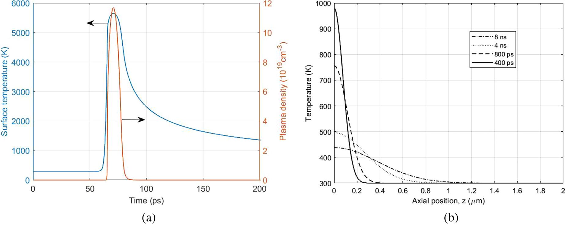
Typical numerical results on the dependence of the temperature on time and position after irradiation with a 7 ps laser pulse are presented in Figures 1(a) and 1(b). The plasma density is directly connected to the temperature of the target surface (presented in Figure 1(a), left-hand side) by relation
${T}_\mathrm{p}=0.67{T}_{z=0,t}$
, which accounts for the Knudsen layer[18,20–22]. The electron density
$n$
is related to the vapour density above the target surface, which is further connected to the saturated vapour density at the surface temperature
${n}_\mathrm{vapour}=0.31{n}_\mathrm{saturated}\left({T}_{z=0,t}\right)$
, which is directly dependent on the saturated vapour pressure
${P}_\mathrm{sat}$
given by Clausius and Clapeyron[18,20–22]. Thus, electron density is connected by the relation
$n=0.31\eta {n}_\mathrm{saturated}$
. The typical time profile of the plasma density is given in Figure 1(a) (right-hand side). The boundary and initial conditions of the heat equation are provided in the following. The initial condition at the beginning of the laser pulse is as follows:
where
${\lambda}_\mathrm{vap}$
and
${\lambda}_\mathrm{boil}$
represent the latent heats of melting and vaporization per unit mass, respectively, and
$v$
is the recession velocity of the front surface due to evaporation, given by the Hertz–Knudsen equation[18,20–22]. The heat equation (1) was solved numerically in MATLAB. For every laser pulse, the integration time for the heat equation was set to about 100
$\tau$
, with a minimum time step of 20 fs. The spatial computational domain was set to a total thickness
$h$
= 100
${l}_\mathrm{T}$
, with a much denser mesh near the front surface (i.e., smaller than 0.1 nm) to accommodate the volumetric laser absorption at this surface.
Figure 1.Simulation results of (a) the time dependence of the surface temperature (left) and plasma density (right) and (b) the spatial profile along the axial direction at different moments after irradiation with a laser pulse with the following parameters: wavelength = 800 nm, pulse duration = 7 ps and peak power density = 24 GW/cm2.
We calculated numerically the temperature of the target surface (see Figure 1(a), for example), and the corresponding recoil pressure
${P}_\mathrm{rec}$
given by Equation (5) of the expanding vapour, as a function of time. The recoil pressure
${P}_\mathrm{rec}$
and the laser pressure are as follows:
and were added to determine the total pressure exerted on the titanium target:
${P}_\mathrm{tot}={P}_\mathrm{rad}+{P}_\mathrm{rec}$
. Our calculations indicate, for example, that when the power density increases above the ablation threshold, which is approximately 20 GW/cm2 for a pulse duration
$\tau$
= 5.1 ps, the recoil pressure due to ablation
${P}_\mathrm{rec}$
makes the main contribution to the total pressure, being approximately three orders of magnitude higher than the radiation pressure
${P}_\mathrm{rad}$
at 200 GW/cm2, in accordance with previous predictions[9].
By multiplying the total pressure
${P}_\mathrm{tot}$
with the laser beam spot area on the target surface (
${A}_\mathrm{spot}$
= 7.0 mm2), we determined the time-dependent total force exerted on the target surface. By time integration of the force, the momentum transferred to the target by one pulse was determined:
Then, the kinetic energy of the target was derived as
${E}_\mathrm{kin}={p}^2/2{m}_\mathrm{target}$
and, by dividing the kinetic energy by the total energy of the laser pulses, we determined the efficiency of the energy transfer. In Figure 2(a), the peak power density is varied by changing the pulse energy in the range of 1–300 mJ, while pulse duration is kept constant at 5.1 ps. In Figure 2(b), the peak power density is varied by changing the pulse duration in the range of 1 μs–1 ps while the pulse energy is kept constant at 30 mJ.
Figure 2.Simulation results of kinetic energy dependence on power density, controlled by: (a) pulse energy between 1 and 300 mJ, = 1064 nm, = 5.1 ps; (b) pulse duration between 1 ps and 1 μs for constant pulse energy = 30 mJ.
In the multi-pulse regime, the simulations were carried considering the spatial distribution of the temperature T(z) from the end of the integration time corresponding to a certain laser pulse (see Figure 1(b)) as the initial condition for the next pulse. When considering the multiple N pulse regime, we calculated the plume length by the product of plasma velocity and total integration time, which is N times
${\tau}_\mathrm{int}$
. Thus, the plasma length is directly related to the pulse number.
3 Experimental system
An inertial pendulum can be considered one of the most reliable methods with sufficient sensitivity to characterize the impulse transferred from a light pulse to a macroscopic target. Following this approach, we built a pendulum with the length
${l}_\mathrm{pen}$
= 120 mm and a metallic foil target with a 10 mm2 area.
To minimize the errors generated from the air–target friction, the system was placed inside a low-vacuum chamber, as presented in Figure 3(a), where the pressure was set to about 0.1 mbar during the experiments, which were all performed at room temperature. During the experiments, the target was irradiated with two types of laser: a high repetition rate ‘Lumera’ Nd-YAG laser, tuneable in the range (400 kHz–1 MHz), delivering laser pulses with fixed pulse duration
$\tau$
$\approx$
7 ps at 1064 nm central wavelength with a high repetition rate
${f}_\mathrm{p}$
, and a high-power laser system (TEWALAS) delivering ultrashort pulses with a tuneable duration from tens of picoseconds (ps) down to tens of femtoseconds (fs) at
${\lambda}_0$
= 800 nm central wavelength and 10 Hz maximum repetition rate. The minimum pulse duration was set by tuning the compressor’s grating distance with a stepper-motorized translation stage using the available commercial SPIDER (APE Berlin, early model with S/N SO2177-O8A6) equipment[28,29] as feedback, while the elongation of the pulse duration up to 5 ps was done by modifying the grating distance within several steps with the unit size calibrated at high distances from the best compression. The pulse energy was measured using a pyroelectric energy detector (GENTEC model 11QE50).
Figure 3.(a) Experimental setup of gravitational pendulum and (b) schematic forces diagram.
The laser beam spot area on target from both lasers was
${A}_\mathrm{spot}$
= 7.0 ± 0.5 mm2. In this experimental configuration, the laser pulses hit the target on a normal incidence, inducing oscillation along a direction parallel with the laser beam.
The target position was recorded using a charge-coupled device (CCD) camera (Basler GigE) placed perpendicular to the pendulum oscillation direction with a fixed frame rate.
Within our experimental approach, by knowing the laser pulse energy
${W}_\mathrm{p}$
, experimentally measured using a standard pyroelectric energy meter, and by measuring the pendulum kinetic energy
${E}_\mathrm{kin}$
, we could evaluate the energy transfer efficiency. By knowing the target mass
$m \approx 25$
mg and pendulum length
${l}_\mathrm{pen}$
, from pendulum deviation
${d}_\mathrm{p}$
, the formula is as follows:
and by further considering energy conservation between potential
${E}_\mathrm{p}$
and kinetic
${E}_\mathrm{kin}$
, the maximal energies are as follows :
where
$v$
is the target velocity and
$g$
is gravitational acceleration constant. We could evaluate the transferred kinetic energy and respectively kinetic energy transfer efficiency
${T}_\mathrm{ef}$
as follows:
The calculation errors of the transfer efficiency (represented as error bars within the graphs) further presented were mostly generated by errors in evaluating pendulum kinetic energy errors from CCD recorded images, and respectively trajectory interpolation, while laser pulse energy measurement is giving considerable smaller possible errors (
$<1\%$
).
4 Results and discussion
Impulse transfer experimental measurements were initially performed on the titanium target for pulses with 7 ps duration, train energies
${W}_\mathrm{train}$
= 426 and 652 mJ and variable repetition rates
${f}_\mathrm{p}$
between 400 and 1000 kHz. By changing the number of pulses
$N$
within a train while keeping the train energy
${W}_\mathrm{train}$
and duration constant, we have also changed ‘effective’ laser–target interaction duration and respectively pulse power density, and the result was a change in the kinetic energy efficiency transfer, as presented in Figure 4(a). These results could be considered ‘predictable’ as long as the laser-thrust efficiency is known to increase with the laser power density[17]. Power density variation in the domain of 1011–1013 W/cm2 was further investigated also by adjusting the laser–matter interaction duration at 30 and 70 mJ single-pulse constant energies, but the resulting trend is an opposite one in this case, as presented in Figure 4(b). Considering the different trends over kinetic energy transfer efficiency for power variations obtained with similar methods (reducing the laser–matter interaction time at constant energies), there is obvious evidence that there should be an ‘optimal’ power density in between the two power ranges, corresponding to a specific pulse duration and energy for a maximal kinetic energy transfer efficiency, as also previously mentioned in other publications[10,11].
Figure 4.Experimental results of kinetic energy transfer efficiency at different beam energies for (a) the multi-pulse ps laser (tuned train frequency from left to right in each series: 1000, 800, 625, 500 and 400 kHz) and (b) the single-pulse fs laser (with tuned duration from left to right in each series: 5100, 4200, 3000, 2100, 1500, 900, 300 and 30 fs).
The single-pulse regime is fundamentally important for understanding the laser–matter interaction and we have experimentally investigated the influences of the main pulse parameters, such as energy, power density and duration, over the kinetic energy transfer efficiency, while preserving the experimental setup and all other parameters constant, including the IR beam wavelength of 800 nm. By comparing the simulated results with the experimental results, we have tried on one hand to check the modelling viability for the simulated experimental conditions and, on the other hand, to identify the optimal experimental condition predicted by the theoretical model.
4.1.1 Single-pulse regime: optimal pulse duration
For understanding the above-presented results, we started by modelling the single-pulse laser–matter interaction experimental results and numerical results on the dependence of transfer efficiency on the pulse duration and pulse power density, at several constant pulse energies, as presented in Figure 5. The laser power density was varied by setting the pulse energy constant (
${W}_\mathrm{p}$
= 10, 30, 50, 70, 90, 110 mJ) and changing the pulse duration in the range of 1 μs–1 ps. Thus, simulations suggest that for fixed pulse energy, the transfer efficiency is very small and constant at a long pulse duration of the order of 1–10 μs, or even more depending on the pulse energy. Further decrease of the pulse duration sets in the ablation process and the strong recoil pressure of the ablation plume lead to an increase of about six to eight orders of magnitude of the transfer efficiency. It should be noticed that the transfer efficiency and the optimal pulse duration are both dependent on the pulse power density, as shown by the simulation results presented in Figure 5(b), which are in good agreement with the experimental data. The results presented in Figure 5(a) indicate that the optimal pulse duration is of the order of a few ps for
${W}_\mathrm{p}$
= 10 mJ, and an increase of pulse energy above
${W}_\mathrm{p}$
= 100 mJ leads to an optimal pulse duration of a few hundred ps. Figure 5(b) indicates a limit value for the transfer efficiency of about 0.001% for laser power density of approximately equal to 5 GW/cm2. It should be also noticed from Figure 5(b) that the ratio of the optimal laser power density to the ablation threshold power density is approximately 500:1 for the pulse energies considered here. This correlation relies on the competition between enhancement of the recoil pressure with laser power density and the enhancement of the plume absorptivity with laser power density, since both processes dominate over the radiation pressure mechanism above the ablation threshold.
Figure 5.Simulation results of kinetic energy transfer efficiency dependence on (a) pulse duration and (b) power density. Experimental data points with error bars of 800 nm laser pulses are represented as blue ( = 30 mJ) and red ( = 70 mJ).
In most real experimental cases, the laser pulse duration is actually the constant value of the system rather than the pulse energy. We started from the fact that even if at power densities of the order 1012 W/cm2, where the increase is based on the pulse duration reduction, the efficiency of the kinetic energy transfer is decreasing, and an increase of the power density based on the increase of the pulse energy in a certain range (up to a few times in our case) gives the opposite trend, as shown in Figure 6(a) for a single laser pulse with duration estimated at 35 fs and pulse energy of up to about 120 mJ in our particular case. It is evident that with the increase of the pulse energy for fixed pulse duration, transfer efficiency increases less and less, and after a value that in our experimental case (for a 35 fs duration and titanium target material) is about 4 × 10¹³ W/cm2, the kinetic energy transfer efficiency starts to decrease. In other words, the increase of the pulse energy should increase the transfer efficiency just within a limited interval. Further experiments were performed for estimating the transfer efficiency dependence on laser power density at different pulse durations within the ps range. Thus, Figure 6(b) presents the influence of a pulse energy increase from 30 to 70 mJ for different laser pulse durations. In all cases, we have an increase in the transfer efficiency with the pulse energy but an increasing trend (the dotted lines in Figure 6(b) represent gradually slowing down with a further increase of the power density and respectively with the decrease of the pulse duration, as suggested in Figure 6(c)).
Figure 6.Experimental results of kinetic energy transfer efficiency variation with pulse energy for (a) fs pulse duration and (b) different pulse durations within the ps range. (c) Transfer efficiency slope variation at different laser power densities for the same pulse energy variations.
Numerical simulations of transfer efficiency dependence on the pulse energy at constant pulse duration are represented in Figure 7(a). They suggest that, in fact, the kinetic energy transfer efficiency does not significantly depend on pulse duration at small pulse energies, corresponding to power densities below the ablation threshold. At higher power densities above the ablation threshold (and respectively shorter pulse duration), the efficiency could reach one to two orders of magnitude higher values for longer pulses (i.e., 5.1 ps duration) as compared to short pulse duration (3 and 1.2 ps, respectively), supporting the experimental efficiency variation trend previously presented. In terms of power density variation (controlled by pulse energy variation at constant pulse duration), Figure 7(b) shows a very small transfer efficiency value, increasing linearly with pulse power density when the laser power density is below the ablation threshold. For a further increase of power density, above the ablation threshold, strong recoil pressure of the ablation plume leads to a magnitude increase up to eight orders of the transfer efficiency, in good agreement with the (bold circles from Figure 7(b)) experimental results. Even if the optimal pulse energy depends on the pulse duration for our experimental conditions, with the increase of the pulse energy there is still about a 500:1 ratio between the optimal power density and the ablation threshold. For our investigated experimental case, simulations suggest an optimal transfer efficiency trend of about 0.0015% for
${I}_0\approx$
500 GW/cm2 power densities, corresponding to a pulse energy
${W}_\mathrm{p}\approx$
200 mJ and several ps pulse duration.
Figure 7.Simulation results of transfer efficiency variation with (a) pulse energy and (b) pulse power density represented for different pulse durations, = 1.2, 3 and 5.1 ps, for a constant pulse energy = 200 mJ; the experimental data from Figure 6(b) are included as (red) triangles (800 nm, = 1.2 ps), (black) circles (800 nm, = 3 ps) and (green) diamonds (800 nm, = 5.1 ps) error bars.
While the single-pulse energy transfer efficiency is fundamentally important, for real (macroscopic) applications, it is very unlikely to be effective since the transferred energy is still relatively low from the macroscopic object point of view, so, it is realistic to consider that trains of pulses should rather be used. In the following experiments, we have studied the influence of certain train parameters on transfer efficiency, such as the number of pulses, repetition frequency and train energy.
4.2.1 Multi-pulse regime: influence of the number of pulses and frequency
Considering the single-pulse kinetic energy transfer optimization, there is a tendency for intuitive extrapolation of the results for a multi-pulse regime. Measurements of transfer efficiency dependence on the number of train pulses using constant beam parameters (in other words, by simply increasing train duration) are presented in Figure 8. From the energetic point of view, the result of increasing the number of pulses will be an increase of the train energy (at constant pulse energy) and the experimental trend looks similar to the single pulse in terms of energy growth influence. Thus, there will be an increase of the efficiency with the number of pulses (and consequently with the train energy), but this increase will tend to reach a maximal value, after which a further increase of the number of pulses will start to decrease the global transfer efficiency. Figure 8 presents curves of transfer efficiency dependence on the number of pulses for several train frequencies at comparable pulse power densities (2–3 MW/cm2). From Figure 8 it should be noticed that even if all the curves have a similar trend of variation with the number of pulses, their global amplitude variation is significantly influenced by the train frequency, rather than the beam (instantaneous) power density. Thus, while further irradiating a titanium target with a 7 ps train pulses at 1064 nm, we used constant average laser power (and respectively average power density). The influence of the train filling factor (respectively repetition rate) is effectively affecting the transferred impulse and respectively transfer efficiency (Figure 9), as expected. This could be easily understood by considering the decrease of the number of pulses in a given train duration and respectively the decrease of the effective laser–matter interaction time. Such reduction of the duration means an increase in the instantaneous power density of the pulses. For a pulse duration of 7 ps and train energies of hundreds of mJ, (instantaneous) power density should still be below the ablation threshold of the titanium, and an increase of the power density should correspond to a quasi-linear increase of the transfer efficiency, as previously presented. We attribute the efficiency transfer decrease for the longer train and highest power (120 ms, 400 kHz) point to some possible measurement errors.
Figure 8.Experimental data on kinetic energy transfer efficiency variation with the number of pulses of 7 ps and 1064 nm, at different laser frequencies, for comparable power densities.
By simulating transfer efficiency versus pulse number
$N$
for the multi-pulse regime, at different pulse energies and frequencies, the obtained numerical results indicate that when maintaining a constant pulse energy
${W}_\mathrm{p}={W}_\mathrm{train}/N$
, the peak temperature increases with the number of pulses during multi-pulse irradiation. However, we should mention that, because of computer resource limitations, we opted for simulating trains with higher energy per pulse (to limit the number of pulses per train), so further presented simulations will have just a qualitative relevance for our experiments. Thus, Figure 10(a) presents the increase of surface peak temperature with pulse number, considering a 4 mJ pulse energy and a succession period between two consecutive pulses
${\tau}_\mathrm{int}$
= 100
$\tau$
. In these conditions, the boiling temperature at the surface is reached after just 10 pulses. For comparison, simulations were also carried out with the same pulse energy and pulse number conditions, considering that the target is cooled down to the original temperature (300 K) before each pulse. The lower (blue) curve (straight line) in Figure 10(a) indicates that the peak temperature is constant when increasing the pulse number and does not reach the melting or boiling points during multi-pulse irradiation. In Figure 10(b), a strong increase of the kinetic energy transfer efficiency of 4 mJ pulses is obtained after just 10 pulses. Numerical results indicate that, even if the first pulses do not produce ablation of the target, after a certain number of laser pulses, the peak temperature of the surface increases above the material boiling values and initiates ablation processes, further leading to a significant increase of the transfer efficiency. For comparison, the blue curve (flat curve) was calculated considering that the target is cooled down to the original temperature before each pulse. The inset plot in Figure 10(b) demonstrates a linear increase of the efficiency with pulse number when cumulative heating of the target is not accounted for. For simulating a train of pulses with twice the repetition frequency (2
${f}_\mathrm{p}$
) of the same laser average power, we set twice as many pulses in the irradiation time train at half the pulse energy
${W}_\mathrm{p}$
and half the integration time. Numerical simulations from Figure 10(c) represent the transfer efficiency dependence on the number of pulses at three frequencies:
${f}_\mathrm{p}$
,
$2{f}_\mathrm{p}$
and
$3{f}_\mathrm{p}$
.
Figure 10.(a) Simulation results of surface peak temperature versus pulse number. (b) Transfer efficiency versus pulse number. The blue curve and the inset plot correspond to ‘cooled’ targets down to 300 K before each consecutive pulse. (c) Transfer efficiency versus pulse number at three working frequencies.
To clarify the origin of the efficiency dependence on frequency, we carried out calculations to determine the dependence of the transfer efficiency on the pulse number and train duration. For that, we considered that during the fixed train duration
${\tau}_\mathrm{train}$
, there are generated
$N$
= 30, 60 and 90 pulses at a succession period between two consecutive pulses
${\tau}_\mathrm{int}$
of 200
$\tau$
, 100
$\tau$
and 70
$\tau$
, respectively, corresponding to three different repetition frequencies (
${f}_\mathrm{p}$
= 1/
${\tau}_\mathrm{int}$
=
$N$
/
${\tau}_\mathrm{train}$
):
${f}_\mathrm{p}$
,
$2{f}_\mathrm{p}$
and
$3{f}_\mathrm{p}$
, respectively. Firstly, we neglected the heat accumulation between consecutive pulses (Figure 11(a)) and, secondly, we accounted for the heat accumulation between consecutive pulses (Figure 11(b)). The results presented in Figure 11(a) indicate that the time interval between the pulses does not influence the transfer efficiency if we neglect the thermal energy accumulation from pulse to pulse. Figure 11(b) demonstrates that, when considering thermal energy accumulation at the same laser energy and pulse number, the efficiency increases by up to eight orders of magnitude when ablation initiates. Figure 11(b) also demonstrates that, when considering thermal energy accumulation, low repetition frequency pulses are more efficient in transferring their energy to the target as compared to high repetition frequency pulses.
Figure 11.Simulation results of the transfer efficiency versus train duration: (a) by neglecting the heat accumulation between pulses and (b) by accounting for the heat accumulation between two consecutive pulses.
A power density increase by increasing the pulse energy
${W}_\mathrm{p}={W}_\mathrm{train}/N$
in a train was investigated at different laser frequencies. Figure 12 indicates that for a given pulse train duration and number of pulses
$N$
, the increase of the train energy
${W}_\mathrm{train}$
induces an increase of the global transfer efficiency. However, the increase of the energy produces a smaller and smaller increase, particularly with the decrease of the laser–matter interaction duration (which is the pulse duration multiplied by the ‘number of pulses’) and respectively the increase of the power density. As can be seen in Figure 12(a), for a 20 ms train duration, the increase of the power density produces a smaller and smaller transfer efficiency increase, regardless whether it was obtained by shortening the laser–matter interaction time (decrease of the number of pulses) or by further increasing the pulse energy. In the inset of Figure 12 is presented the slope variation trend with the power density, for different frequencies (number of pulses) in the train with 20 ms duration. From an application point of view, if for a single pulse this corresponds in our case to about a 500:1 power density ratio with the ablation threshold, in the case of the multi-pulse regime, it should correspond to an optimal number of ablated particles, generated by the train pulses in the given experimental conditions. The numerical results obtained in the multi-pulse regime on the dependence of transfer efficiency on the laser peak power density are presented in Figure 12(b). We simulated two different repetition frequencies,
${f}_\mathrm{p}$
and 2
${f}_\mathrm{p}$
, considering that the total energy of the pulse train is divided into
$N$
= 10 and
$N$
= 20 pulses, respectively. Here, the total energy of the pulse train
${W}_\mathrm{train}$
is varied in the range 0.15–2 J, resulting in a pulse energy
${W}_\mathrm{p}$
= 15–200 mJ/pulse when
$N$
= 10, and 7.5–100 mJ/pulse when
$N$
= 20.
Figure 12.(a) Experimental results of the power density influence on kinetic energy transfer efficiency for 20 ms trains of 7 ps pulses (1064 nm); inset, power density influence on slope variation. (b) Numerical results of the dependence of transfer efficiency on the pulse power density.
Similar experimental results were obtained for other different train durations as well, and comparative results for train durations of 20, 40, 80 and 120 ms, train energies
${W}_\mathrm{train}$
of several hundreds of mJ and different pulse frequencies
${f}_\mathrm{p}$
are presented in Figure 13. It could be observed that an increase in train energy produces in all cases an increase of the kinetic energy transfer efficiency. However, at a shorter train duration, the saturation of the transfer efficiency increase occurs at smaller energies, while for power densities around 5 MW/cm2, a further increase of train energy is already inducing a decreasing trend in the transfer efficiency variation after several tens of ms train duration, corresponding in our experimental cases to tens of thousands of pulses.
Figure 13.Experimental results of kinetic energy transfer efficiency variation with power density for different train energies at (a) 20 ms, (b) 40 ms, (c) 80 ms and (d) 120 ms train duration.
Considering the hypothesis of the simulations and their correspondence with the experimental results, we could draw some conclusions on the optimal number of pulses per train. That specific number should correspond to optimal ablation conditions, which in our approximations rely on reaching a specific target surface temperature dependent on the heat accumulation process; a comparable amount of heat in the same time interval would be obtained by double the number of pulses of half energy. In other words, for a double operating frequency, the optimal energy transfer should correspond to double the number of pulses with a half-power density. Thus, considering the heat accumulation in the target as the dominant factor in initiating the ablation process and, consequently, as the kinetic energy transfer buster process, a generic variation formula of the optimal number of pulses per train dependence on train frequency and train energy should be given by the following:
where
${f}_\mathrm{p}$
is the train repetition frequency,
${W}_\mathrm{train}$
is the train energy and
${k}_\mathrm{p}$
is a proportionality constant depending on the ablation process parameters, such as the laser wavelength, pulse duration, material absorption coefficient at the laser wavelength and respectively the ablation threshold for the specific wavelength, pulse duration and heat conductivity of the target material.
From an application point of view, this limitation of the transfer efficiency has clear importance. Thus, for a given (laser) pulse duration there is an optimal pulse energy and respectively an optimal number of pulses (in correlation with the laser frequency) for an optimal transfer efficiency, after which the efficiency of the injected energy will start decreasing. In other words, the transfer efficiency will increase with the total number of pulses and their energy, but, after a certain point, supplementary injected energy influence becomes neglectable or even starts diminishing the global efficiency of the transferred kinetic energy.
5 Conclusions
In conclusion, we could summarize that our experimental studies on an inertial pendulum with Ti targets combined with the theoretical simulations based on heat and photon energy transfer and respectively photon reflection have shown a kinetic energy transfer efficiency optimal value for beam power densities about 500 times larger than the ablation threshold values, corresponding in our case to an optimal pulse duration of tens to hundreds of ps. Consequently, the optimal pulse energy for a given pulse duration and beam diameter is the energy providing a power density on the target that is 500 times higher than the ablation threshold. For the case of multi-pulse regimes, as a more effective approach than laser-thrust applications, there is a more efficient transfer from lower repetition rate train pulses than from higher rates. Increasing the train energy is in principle increasing transfer efficiency but within a limited variation range, while the optimal number of pulses per train depends proportionally on the repetition rate and inverse proportionally on the beam power density (and respectively pulse energy). The proportionality constant depends on the target material and other beam parameters. In our experimental case of the Ti target, 7 ps IR laser pulse duration,
$\unicode{x3bc}\mathrm{J}$
energies per pulse and repetition rates of hundreds of MHz, the optimal number of pulses is in the range of tens to few hundreds of thousands of pulses per train, while the maximal transfer efficiency could reach values of about 0.0015%.
References
[1] X.-T. Zhao, F. Tang, B. Han, X.-W. Ni. J. Appl. Phys., 120, 213103(2016).
[2] P. Battocchio, J. Terragni, N. Bazzanella, C. Cestari, M. Orlandi, W. J. Burger, R. Battiston, A. Miotello. Measurem. Sci. Technol., 32, 015901(2020).
[3] B. D’Souza, A. Ketsdever35th AIAA Plasmadynamics and Lasers Conference. and , in (American Institute of Aeronautics and Astronautics, ), paper AIAA 2004-2664.(2004).
[4] M. J.-E. Manuel, T. Temim, E. Dwek, A. M. Angulo, P. X. Belancourt, R. P. Drake, C. C. Kuranz, M. J. MacDonald, B. A. Remington. High Power Laser Sci. Eng., 6, e17(2018).
[5] B. Nasseri, E. Alizadeh, F. Bani, S. Davaran, A. Akbarzadeh, N. Rabiee, A. Bahador, M. Ziaei, M. Bagherzadeh, M. R. Saeb, M. Mozafari, M. R. Hamblin. Appl. Phys. Rev., 9, 011317(2022).
[6] T. Nakamura, Y. Herbani, D. Ursescu, R. Banici, R. V. Dabu, S. Sato. AIP Adv., 3, 082101(2013).
[7] H. Ahn, I. Jun, K. Y. Seo, E. K. Kim, T.-I. Kim. Sci. Rep., 12, 10656(2022).
[8] P. N. Lebedev. Ann. Phys, 6, 433(1901).
[9] A. Kantrowitz. Astronaut. Aeronaut., 10, 74(1972).
[10] V. H. Shui, L. A. Young, J. P. Reilly. AIAA J., 16, 649(1978).
[11] B. Esmiller, C. Jacquelard, H.-A. Eckel, E. Wnuk. Appl. Opt., 53, I45(2014).
[12] C. R. Phipps, M. Boustie, J. M. Chevalier, S. Baton, E. Brambrink, L. Berthe, M. Schneider, L. Videau, S. A. E. Boyer, S. Scharring. J. Appl. Phys., 122, 193103(2017).
[13] G. Wang, J. Sun, P. Ji, J. Hu, J. Sun, Q. Wang, Y. Lu. J. Phys. D, 53, 165104(2020).
[14] R. Ecault, L. Berthe, F. Touchard, M. Boustie, E. Lescoute, A. Sollier, H. Voillaume. J. Phys. D, 48, 095501(2015).
[15] I. J. Kim, K. H. Pae, I. W. Choi, C.-L. Lee, H. T. Kim, H. Singhal, J. H. Sung, S. K. Lee, H. W. Lee, P. V. Nickles, T. M. Jeong, C. M. Kim, C. H. Nam. Phys. Plasmas, 23, 070701(2016).
[16] T. Esirkepov, M. Borghesi, S. V. Bulanov, G. Mourou, T. Tajima. Phys. Rev. Lett., 92, 175003(2004).
[17] S. S. Harilal, J. R. Freeman, P. K. Diwakar, A. Hassanein. Laser-Induced Breakdown Spectroscopy: Theory and Applications, 143(2014).
[18] M. Stafe, C. Negutu. Plasma Chem. Plasma Process., 32, 643(2012).
[19] N. M. Bulgakova, A. V. Bulgakov. Appl. Phys. A, 73, 199(2001).
[20] S. Amoruso, M. Armenante, V. Berardi, R. Bruzzese, N. Spinelli. Appl. Phys. A, 65, 265(1997).
[21] M. Stafe. J. Appl. Phys., 112, 123112(2012).
[22] M. Stafe, A. Marcu, N. N. Puscas. Pulsed Laser Ablation of Solids: Basics, Theory and Applications(2013).
[23] E. G. Gamaly, B. Luther-Davies, V. Z. Kolev, N. R. Madsen, M. Duering, A. V. Rode. Laser Particle Beams, 23, 167(2005).
[24] T. W. Murray, J. W. Wagner. J. Appl. Phys., 85, 2031(1999).
A. Marcu, M. Stafe, M. Barbuta, R. Ungureanu, M. Serbanescu, B. Calin, N. Puscas. Photon energy transfer on titanium targets for laser thrusters[J]. High Power Laser Science and Engineering, 2022, 10(5): 05000e27

 = 800 nm, pulse duration
  = 7 ps and peak power density
  = 24 GW/cm2.
 dependence on power density, controlled by: (a) pulse energy
  between 1 and 300 mJ,
  = 1064 nm,
  = 5.1 ps; (b) pulse duration
  between 1 ps and 1 μs for constant pulse energy
  = 30 mJ.
 = 30 mJ) and red (
 = 70 mJ).
 fs pulse duration and (b) different pulse durations within the ps range. (c) Transfer efficiency slope variation at different laser power densities for the same pulse energy variations.
 = 1.2, 3 and 5.1 ps, for a constant pulse energy
  = 200 mJ; the experimental data from Figure 6(b) are included as (red) triangles (800 nm,
  = 1.2 ps), (black) circles (800 nm,
  = 3 ps) and (green) diamonds (800 nm,
  = 5.1 ps) error bars.
 : (a) 8.15 W; (b) 10.2 W; (c) 14.55 W.