• High Power Laser Science and Engineering
  • Vol. 9, Issue 4, 04000e64 (2021)
M. Scisciò1、*, F. Consoli1, M. Salvadori1, N. E. Andreev2、3, N. G. Borisenko4, S. Zähter5、6, and O. Rosmej5、6
Author Affiliations
  • 1ENEA, Fusion and Technologies for Nuclear Safety Department, 00044Frascati, Italy
  • 2Joint Institute for High Temperatures, Russian Academy of Sciences, 125412Moscow, Russia
  • 3Moscow Institute of Physics and Technology (National Research University), 141701Moscow, Russia
  • 4P. N. Lebedev Physical Institute, Russian Academy of Sciences, 119991Moscow, Russia
  • 5GSI Helmholtzzentrum für Schwerionenforschung GmbH, 64291Darmstadt, Germany
  • 6Goethe University Frankfurt, 60438 Frankfurt am Main, Germany
  • show less
    DOI: 10.1017/hpl.2021.50 Cite this Article Set citation alerts
    M. Scisciò, F. Consoli, M. Salvadori, N. E. Andreev, N. G. Borisenko, S. Zähter, O. Rosmej. Transient electromagnetic fields generated in experiments at the PHELIX laser facility[J]. High Power Laser Science and Engineering, 2021, 9(4): 04000e64 Copy Citation Text show less

    Abstract

    Large-amplitude electromagnetic radiofrequency fields are created by the charge-separation induced in interactions of high-intensity, short-pulse lasers with solid targets and have intensity that decreases with the distance from the target. Alternatively, it was experimentally proved very recently that charged particles emitted by petawatt laser–target interactions can be deposited on a capacitor-collector structure, far away from the target, and lead to the rapid (nanosecond-scale) generation of large quasi-static electric fields ($\mathrm{MV}/\mathrm{m}$), over wide regions. We demonstrate here the generation of both these fields in experiments at the PHELIX laser facility, with approximately $20\;\mathrm{J}$ energy and approximately ${10}^{19}\;\mathrm{W}/\mathrm{c}{\mathrm{m}}^2$ intensity, for picoseconds laser pulses, interacting with pre-ionized polymer foams of near critical density. Quasi-static fields, up to tens of kV/m, were here observed at distances larger than $1\;\mathrm{m}$ from the target, with results much higher than the radiofrequency component. This is of primary importance for inertial-confinement fusion and laser–plasma acceleration and also for promising applications in different scenarios.

    1 Introduction

    High-power laser systems (from the GW up to the PW range) are used for performing laser–plasma interaction experiments, exploiting the interaction of focused high-intensity laser pulses with solid targets. These experiments aim at studying various fields of physics, such as laser-driven particle acceleration[1], laboratory astrophysics[24] and the ion-driven fast ignition approach for inertial confinement fusion[5]. One of the consequences of the laser–target interaction is the generation of pulsed electromagnetic (EM) fields (electromagnetic pulses, EMPs)[6,7]. The mechanisms that drive these EMPs can be different – depending on the interaction regime – and EM radiation with associated different features can be thus emitted at different intensities (up to several MV/m) and frequencies (from the MHz to the THz range)[6,7]. The most well-known EMP emission mechanism is related to the neutralization current that flows through the target holder due to the laser pulse depleting the solid target from electrons[812]. This leads to the generation of a fast-oscillating, radiated EM field in the range of radiofrequencies (RFs), that is, from megahertz up to a few gigahertz, that propagates inside the vacuum chamber and also is capable of reaching the space external to the chamber. The amplitude of the electric field can reach the order of megavolts per meter and it represents one main hazard for electronic devices nearby, due to efficient EM coupling in this frequency range. However, intense electric fields can also be generated by the charged particles that are emitted from the irradiated target[7,1315]: ion wakefields and charge accumulation on surrounding objects can lead to intense quasi-static fields that superimpose on the RF EMP signal. In Ref. [14], Consoli et al. reported measurements performed at the Vulcan PW laser facility, where electrons and protons impinged onto the focusing parabola of the experimental laser setup, which led to transient electric fields in the range of hundreds of kilovolts per meter at a distance of a few meters from the interaction point. In this paper, we present experimental data that exhibit similar characteristics to those reported in Ref. [14], which were obtained during a campaign at the PHELIX laser facility (GSI, Germany)[16]. Our measurements represent a further confirmation that particles emitted from the target are capable of accumulating on objects in the vacuum chamber and therefore generate transient quasi-static electric fields. Moreover, this type of EMP is capable of generating extremely high electric fields at large distances from the target (a distance of over $1\;\mathrm{m}$, in our case), while the classical RF EMPs, driven by the neutralization current through the target holder, have their amplitude decreased significantly[810]. This makes the study of such EMPs very important for the implementation of electronic equipment in existent and upcoming laser facilities for both laser–plasma acceleration[1719] and inertial confinement fusion[17,20,21]. By implementing a D-dot differential E-field probe[22], we measured a quasi-static electric field localized between a Teflon brick – which was irradiated by ions and electrons stemming out of the target – and the conducting external chamber wall, which acts as an open capacitor-collector structure. At the position where our field probe was placed, the quasi-static field and the RF component combined for an amplitude in the multiple tens of kV/m order. Using a methodology similar to the one used in Ref. [14], we studied the temporal evolution of the electric field signal with particle-in-cell (PIC) simulations. The numerical results indicate that the quasi-static electric field is generated by the combination of the following. (1) Ion wakefields, that is, the static electric field that is associated with drifting ions: being non-relativistic, the resulting fields have both a longitudinal (i.e., in the direction of motion of the particles) and a transversal components[23,24]. (2) Charge accumulation, due to accelerated ion populations with different mean energies that irradiate the Teflon object inside the chamber.

    2 Experimental results

    The measurements presented here were obtained during a campaign at the PHELIX laser system (located at the GSI research facility in Germany), which provided – in our specific setup, reported in Figure 1 – pulses with duration of $\tau \approx 750\;\mathrm{fs}$ and energy up to approximately $100\;\mathrm{J}$ after the compressor and about 20 J within the full width at half-maximum (FWHM) focus on the target. The laser light (S-polarized, $\lambda = 1053\;\mathrm{nm}$ wavelength) was focused down with an off-axis parabola on a solid target (rotated by ${7}^{\circ }$ from the laser axis, made of a CHO 2 mg/cc polymer foam of $350\;\unicode{x3bc} \mathrm{m}$ thickness stacked with a $1\;\mathrm{mm}$ thick Au planar converter from the rear side), yielding an intensity of ${I\approx 2.5\times {10}^{19}\;\mathrm{W}/\mathrm{c}{\mathrm{m}}^2}$ on a spot of approximately $15\;\unicode{x3bc} \mathrm{m}$ FWHM. Prior to the main pulse, a secondary pulse, with a delay of $2.5\;\mathrm{ns}$ and an energy of $1\;\mathrm{J}$, irradiated the target for pre-ionizing the foam layer and created a plasma of near critical density [25]. As reported in Figure 1, the area in the laser forward direction, in front of the target, was devoted to diagnostics for measuring the energy, the spectra and the spatial distribution of relativistic electrons generated in the foam and gamma radiation in Au-converter, the main purpose of the campaign[25]. A characteristic feature of laser interaction with a plasma of near critical density, is the production of high current electron and ion beams. At an angle of ${80}^{\circ }$ from the laser axis, and at a distance of ${d}_{\mathrm{Ddot}} = 123\;\mathrm{cm}$, we placed a D-dot differential probe (which is pictured in the photograph of Figure 1) for measuring the electric field of the laser-driven EMP signal[6]. A $10\;\mathrm{cm}$ thick Teflon brick ($30\;\mathrm{cm}$ wide and $30\;\mathrm{cm}$ high) was placed between the field probe and the laser–plasma interaction point – at a distance of ${d}_{\mathrm{T}} = 95\;\mathrm{cm}$ from the target – with the purpose of shielding the D-dot from direct particle and ionizing EM irradiation (e.g., ultraviolet (UV)-X-rays). The D-dot, which measures the component of the electric field along its sensitive axis (see the photograph in Figure 1), was orientated in such a way to measure the ${\overrightarrow{E}}_{\kern-1.5pt{z}}$ component of the electric field in the reference system reported in the setup scheme (Figure 1). We estimate the eventual misalignment of the probe to be not greater than $\pm {10}^{\circ }$ with respect to the $z$-axis, that is, leading to an uncertainty lower than 2% for the measured signal amplitude. The differential signal, which is proportional to the time-derivative of the incident electric field, was transformed by a balun[22] to a single-channel signal, and then transmitted to a Lecroy WP 735Zi (4 GHz) oscilloscope through an approximately $10\;\mathrm{m}$ long, double-shielded coaxial cable. A time-of-flight (TOF) diamond detector[26] was installed at an angle of ${90}^{\circ }$ from the laser axis, ${d}_{\mathrm{D}} = 152\;\mathrm{cm}$ away from the target, behind the position of the D-dot and elevated above the Teflon wall, in order to obtain information about the ions that were accelerated in the direction of the field probe.

    Experimental setup during the campaign. The focused laser pulse irradiated the solid target, tilted by with respect to the laser axis. Electron and -ray diagnostics were placed in the laser forward direction, whereas the EMP field probe was placed at about from the laser axis at a distance of 123 cm from the interaction point. The ions accelerated by the interaction were detected by means of a diamond TOF diagnostic that was elevated above the Teflon ( from the laser axis, 152 cm away from the target). The photograph shows the D-dot probe used in the experiment.

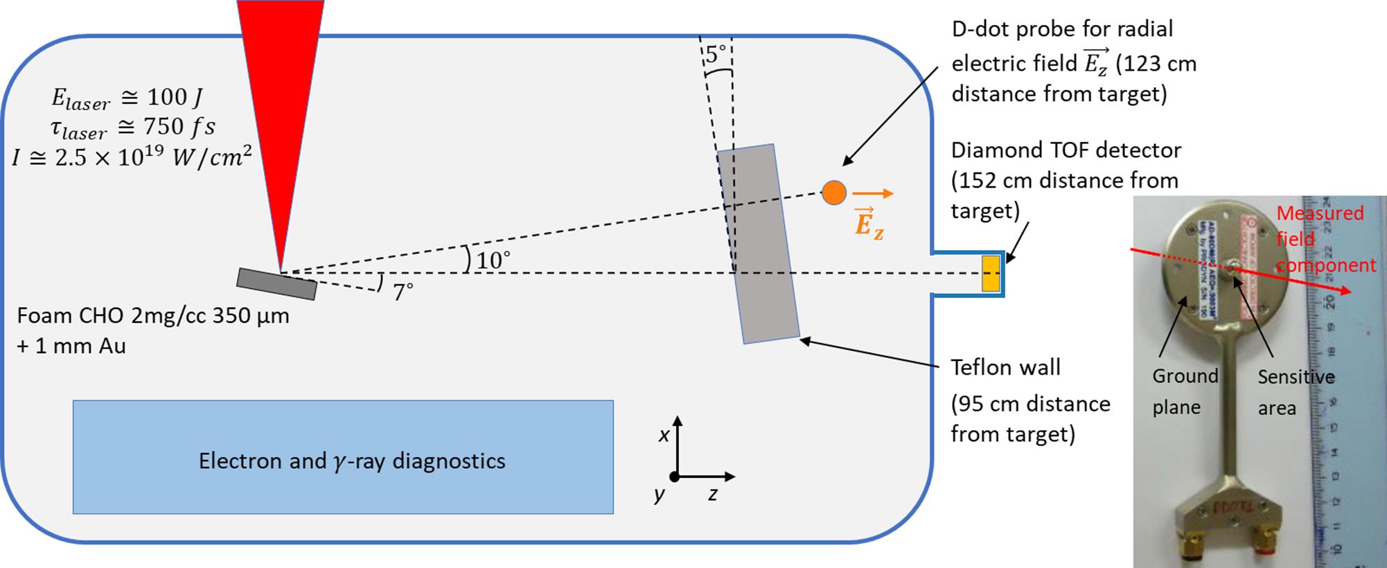
    Figure 1.Experimental setup during the campaign. The focused laser pulse irradiated the solid target, tilted by with respect to the laser axis. Electron and -ray diagnostics were placed in the laser forward direction, whereas the EMP field probe was placed at about from the laser axis at a distance of 123 cm from the interaction point. The ions accelerated by the interaction were detected by means of a diamond TOF diagnostic that was elevated above the Teflon ( from the laser axis, 152 cm away from the target). The photograph shows the D-dot probe used in the experiment.

    In Figure 2(a) we show the raw signal that was retrieved by the D-dot for shot #32 of the campaign, which had a laser energy of $19.3\;\mathrm{J}$ on target. We obtained the reported measurement by acquiring the D-dot signal on two channels of the oscilloscope (using a calibrated signal splitter), set with different amplitude scales, in order to improve the signal-to-noise ratio of the signal (using the same technique reported in Ref. [26]). The frequency-dependent signal attenuation, provided by the cable chain that connected the probe to the scope, was taken into account by performing a de-embedding procedure of the cables and adjusting the retrieved raw signal accordingly (see Section 4.1, devoted to measurement techniques, for details). The signal shown in Figure 2(a), at first glance, is coherent with the temporal shape of a classical laser-driven EMP signal: a fast rise at the moment when the EM signal reaches the probe, followed by megahertz–gigahertz oscillations with an exponentially decaying envelope[10,2730]. It is worth noting that we used a shifted timescale by setting the instant ${t}_0 = 0\;\mathrm{ns}$ at the moment when the rise of the signal occurs (the EM signal takes the propagation time of $t = \frac{d_{\mathrm{Ddot}}}{c}\approx 4.1\;\mathrm{ns}$ to reach the probe, from the moment when the laser–plasma interaction occurs). The numerically obtained Fourier transform of the signal, reported in Figure  2(b), is also compatible with the classical EMP frequency range: a broadband spectrum covering the megahertz–gigahertz range (note that the abrupt cut-off at 4 GHz is due to the oscilloscope bandwidth limitation). In terms of the signal-to-noise ratio, the retrieved signal had an $\mathrm{SNR}>10$ up to about $t = 300\;\mathrm{ns}$. This was achieved by estimating the noise level, so the amplitude of the detected signal, before the rise of the main EMP signal, that is, for $t<-50\;\mathrm{ns}$ in Figure 2(a), resulting ${V}_{\mathrm{noise}}\approx 0.04\;\mathrm{V}$. Hence, from these measurements we chose to reconstruct the electric field, as explained in the following, up to this time value, in order to ensure a high accuracy of our obtained field.

    (a) Time domain signal retrieved by the D-dot probe for shot #32. The timescale has been adjusted in order to overlap t = 0 with the initial rise of the main EMP signal. The small signal at t f = 4 GHz is due to the bandwidth limitation of the oscilloscope.

    Figure 2.(a) Time domain signal retrieved by the D-dot probe for shot #32. The timescale has been adjusted in order to overlap t = 0 with the initial rise of the main EMP signal. The small signal at t < 0 is likely due to the laser pre-pulse impinging the target. (b) Frequency domain signal, obtained by the numerical fast Fourier transform of the D-dot time signal. The cut-off at f = 4 GHz is due to the bandwidth limitation of the oscilloscope.

    The temporal evolution of the electric field needs to be reconstructed from the D-dot signal by numerical time integration[14]:

    $$\begin{align} {E}_{\mathrm{n}}(t) = {K}_{\mathrm{DDOT}}\;{\int}_0^t{V}_{\mathrm{DDOT}}\left(\tau \right) \mathrm{d}\tau, \end{align} $$ 

    where ${V}_{\mathrm{DDOT}}$ is the raw time signal of the probe reported in Figure 2(a) and ${K}_{\mathrm{DDOT}} = 9.5\times {10}^{12}\;\mathrm{m}/\mathrm{s}$ is a proportionality factor that also includes the attenuation of the balun. The obtained electric field is reported in Figure 3(a), where we show the measurements of two consecutive shots of the campaign (#32 and #33). In shot #32, the field probe had its sensitive axis oriented along the component ${\overrightarrow{E}}_{\kern-1.5pt{z}}$ of the electric field; in particular, the probe signals were positive for fields pointed towards the chamber wall, as depicted in Figure 1. In shot #33, the probe was intentionally rotated by ${180}^{\circ }$, with the resulting probe signals being negative for fields pointing towards the chamber wall. The laser energy was $19.3\;\mathrm{J}$ in shot #32 and $21.8\;\mathrm{J}$ in shot #33. The time evolution of the field indicates that two EMP generation mechanisms occurred in both shots. The oscillating RF component, which modulates the signal, is due to the ‘classical’ EMP generation mechanism, provoked by the neutralization current flowing through the target holder/structure[812]. This RF component propagated throughout the chamber, reaching the field probe: in both shots, it reached a maximum amplitude of ${E}_{\mathrm{RF}}^{\mathrm{max}}\approx 22\;\mathrm{kV}/\mathrm{m}$ (peak-to-peak value of the fast oscillations, compatible with the scaling reported in Ref. [6], specifically with what was measured at LULI 2000 with ps pulses) at the early times of the signal, that is, right after the interaction moment. The signal then exponentially decreased for longer times, coherently with the raw D-dot signal of Figure 2(a). In particular, in shot #32, $250\;\mathrm{ns}$ after the initial rise at $t = 0$, the high-frequency oscillations have a peak-to-peak value of approximately $3\;\mathrm{kV}/\mathrm{m}$. The measurements show that, in both shots, the temporal evolution of the electric field also exhibits a low-frequency transient growth, occurring over a much longer timescale compared to the typical oscillation period of the RF modulation (i.e., over a temporal lapse of a few hundreds of nanoseconds). The growth of the transient electric field begins at $t = 0$ and reaches at $t\approx 200\;\mathrm{ns}$ a maximum value of ${E}_{\mathrm{T}}^{\mathrm{max}}\approx 58\;\mathrm{kV}/\mathrm{m}$ in shot #32, and at $t\approx 140\;\mathrm{ns}$ a maximum value of ${E}_{\mathrm{T}}^{\mathrm{max}}\approx 72\;\mathrm{kV}/\mathrm{m}$ in shot #33. The transient electric field dominates over the classical RF EMP, being the factor ${E}_{\mathrm{T}}^{\mathrm{max}}/{E}_{\mathrm{RF}}^{\mathrm{max}}\approx 3$ in both shots. This behavior, which is consistent with what is reported by Consoli et al.[14], is stressed by the visualization of Figure 3(b), where the RF component ${E}_{\mathrm{RF}}(t)$ and the quasi-static transient component ${E}_{\mathrm{T}}(t)$ of shot #32 are plotted separately. These signals have been obtained by numerical filtering of the ${E}_{{z}}(t)$ signal of Figure 3(a). The blue plot of Figure 3(b) has been obtained by applying a high-pass finite impulse response (FIR) filter (cut-off frequency ${f}_{\mathrm{c}} = 100\;\mathrm{MHz}$, order $N = 200)$. The red plot has been obtained by applying a low-pass FIR filter (cut-off frequency ${f}_{\mathrm{c}} = 100\;\mathrm{MHz}$, order $N = 287)$. The presence of a strong quasi-static component of the electric field (i.e., the transient component ${E}_{\mathrm{T}}$), as we will discuss more specifically in the following, is due to the interplay of particle wakefield effects from particles stemming out of the laser-irradiated target and charge deposition on the Teflon wall that was placed in front of the field probe. The sign of the retrieved field, that is, a positive field in shot #32 where the D-dot sensitive axis was oriented towards the external chamber wall and a negative field in shot #33 where the probe was intentionally overturned by ${180}^{\circ }$, indicates that the main contribution is due to positively charged particles. The Teflon surface acts, in combination with the external chamber wall, as an open capacitor structure where positive charge is deposited: the resulting electric field has its main component along the $z$ direction (see the coordinate system of Figure 1) and is detected by the D-dot as positive (shot #32) or negative (shot #33, with inverted probe), depending on the orientation of the probe. This model is visually represented by the sketch in Figure 4(a).

    (a) Electric field () as a function of time, reconstructed from the time signal of the D-dot probe placed between the Teflon and the external chamber wall. The E-fields for shots # 32 (blue plot) and #33 (orange plot) are reported. The laser energy was 19.3 and 21.8 J, respectively. The transient component of the field dominates over the RF oscillations in both cases. (b) The RF component () and the transient component () of shot #32, plotted separately. The signals have been obtained from the signal of panel (a) by applying a low-pass FIR filter (for the transient component) and a high-pass FIR filter (for the RF component).

    Figure 3.(a) Electric field () as a function of time, reconstructed from the time signal of the D-dot probe placed between the Teflon and the external chamber wall. The E-fields for shots # 32 (blue plot) and #33 (orange plot) are reported. The laser energy was 19.3 and 21.8 J, respectively. The transient component of the field dominates over the RF oscillations in both cases. (b) The RF component () and the transient component () of shot #32, plotted separately. The signals have been obtained from the signal of panel (a) by applying a low-pass FIR filter (for the transient component) and a high-pass FIR filter (for the RF component).

    (a) Schematic sketch of the charge accumulation effect that occurs on the frontal face of the Teflon. The accelerated protons generate a positive quasi-static charge on the Teflon that, in combination with the chamber wall, acts as a capacitor plate, generating the measured field. (b) Typical proton spectrum obtained during the experimental campaign at from the laser axis, that is, behind the D-dot probe. (c) Top: the temporal evolution of (shot #32) divided into temporal intervals that are associated with the proton populations that were routinely accelerated during the experiment. Below: the TOF signal obtained with the diamond detector placed behind the D-dot. (d) Top: the temporal evolution of (shot #33) divided into temporal intervals that are associated with the proton populations that were routinely accelerated during the experiment. Below: the TOF signal obtained with a diamond detector placed behind the D-dot.

    Figure 4.(a) Schematic sketch of the charge accumulation effect that occurs on the frontal face of the Teflon. The accelerated protons generate a positive quasi-static charge on the Teflon that, in combination with the chamber wall, acts as a capacitor plate, generating the measured field. (b) Typical proton spectrum obtained during the experimental campaign at from the laser axis, that is, behind the D-dot probe. (c) Top: the temporal evolution of (shot #32) divided into temporal intervals that are associated with the proton populations that were routinely accelerated during the experiment. Below: the TOF signal obtained with the diamond detector placed behind the D-dot. (d) Top: the temporal evolution of (shot #33) divided into temporal intervals that are associated with the proton populations that were routinely accelerated during the experiment. Below: the TOF signal obtained with a diamond detector placed behind the D-dot.

    The presence of accelerated protons (from kiloelectronvolt energy up to multiple megaelectronvolts) and ions, in both laser forward and backward directions, having a broad angular distribution especially for the low-energy part of the spectrum, is compatible with the acceleration regimes that are typical at laser intensities of $I>{10}^{18}\;\mathrm{W}/\mathrm{c}{\mathrm{m}}^2$[3135]. Specifically in our case, ions that travel towards the Teflon and the D-dot are clearly observed in the measurements performed with the diamond TOF detector that was placed behind the field probe (see the setup sketch in Figure 1). We placed this diagnostic behind the field probe in order to obtain a reliable estimate of the accelerated particles in proximity of the D-dot. In Figure 4, we discuss the temporal evolution of shots #32 and #33 by comparing the timescale of the transient electric fields (top plots of Figures 4(c) and 4(d), respectively, for #32 and #33) with the TOF signal from the diamond detector (bottom plots of Figures 4(c) and 4(d)) and the retrieved spectrum (Figure 4(b)). The spectrum represents the case where proton populations (but not other ion species) – accelerated by the laser–plasma interaction – generate the TOF signal. The diamond detector was placed along a direction close to the D-dot (see Figure 1). In the case of shot #32, for the time lapse that we indicated with (a) in Figure 4(c), that is, for time from $t = 0$ to $t\approx 40\;\mathrm{ns}$, the rise of the electric field can be due to one or both of the following: (i) ionizing EM radiation emitted from the target (e.g., UV- and X-rays) that interacts with the Teflon wall and that ionizes its frontal surface, leaving a positive net charge that generates the electric field with ${\overrightarrow{E}}_{\kern-1.5pt{z}}$ as the main component, directed towards the external chamber wall; (ii) the accelerated particles emitted from the target travel towards the probe, carrying a ion wakefield that is sensed by the D-dot and grows larger when the particles get closer. For the latter, the positive sign of the electric field indicates that the main contribution is due to a positive net charge associated with the ion bunch. For the time interval (b), that is, from $t\approx 40$ ns to $t\approx 80\;\mathrm{ns}$, it is possible to make a direct comparison with the typical TOF signal obtained with the diamond detector placed behind the D-dot (bottom plot of Figure 4(c)). In order to compare this signal with the temporal evolution of the electric field (top plot of Figure 4(c)), we normalized the timescale of this figure by the factor ${d}_{\mathrm{T}}/{d}_{\mathrm{D}}$: by doing so, the time values of the TOF signal consider the distance from the interaction point to the Teflon. Thus, ions propagate towards the field probe and collide with the Teflon wall at ${d}_{\mathrm{T}} = 95\;\mathrm{cm}$ distance from the interaction point. At $t = 0$ the photo-peak, which is due to ionizing radiation reaching the detector, is recognizable and can be used as a reference time for the laser–plasma interaction moment (for this signal, the timescale is shifted by $ = \frac{d_{\mathrm{D}}}{c}\approx 5\;\mathrm{ns}$). From the photo-peak up to $t = 40\;\mathrm{ns}$ there is no presence of an ion signal. Thus, the field growth of the time span (a) cannot be associated with particle deposition on Teflon, but instead is due to ion wakefield effects. Then, in the time span between $t = 40\;\mathrm{ns}$ and $t = 80\;\mathrm{ns}$, ion populations are visible: the peak around $t\approx 50\;\mathrm{ns}$ corresponds to megaelectronvolt protons, while the later peaks are likely generated by both lower energy proton populations and heavy ions. The time interval (b) of the EMP field signal overlaps with the peaks of the TOF signal (where multiple ion populations are visible). This indicates that the electric field growth of shot #32, during the time span (b), is likely due to a combination of ion wakefield effects and charge accumulation on the Teflon. Indeed, the slope of the electric field is higher in this time interval. In Figure 4(b) we report the ion spectrum obtained from the TOF signal, in the scenario where this is entirely generated by protons[26,36]. The accelerated protons that propagate in direction of the D-dot routinely have energies up to a few megaelectronvolts. In the specific case that we report here, the maximum energy of $2.5\;\mathrm{MeV}$ corresponds to a TOF of approximately $40\;\mathrm{ns}$ from the interaction point to the position of the Teflon wall. The protons with the lowest energy that were detected, that is, $0.8\;\mathrm{MeV}$, take approximately $80\;\mathrm{ns}$ to travel from the target to the Teflon. By applying this methodology to the time interval (c), which lasts up to $t = 200\;\mathrm{ns}$, we obtain protons with energies between $0.8$ and $0.1\;\mathrm{MeV}$ (or heavier and more energetic ions with the same velocity) that are responsible for this final rise of the electric field. As in the most common laser-driven ion acceleration mechanisms (e.g., the target normal sheath acceleration (TNSA)[1]), these were certainly present, but were not detected by the diamond sensor, since it was shielded with an Al foil giving an artificial cut to these low-energy particles. The last time interval (d), that is, for $t>200\;\mathrm{ns}$, corresponds to protons and other ions with energies below $100\;\mathrm{keV}/\mathrm{amu}$. The electric field does not grow in this time interval but rather keeps a quasi-static amplitude. As for the previous time spans, a part of the accelerated ions accumulates on the Teflon, which leads to the static field that was detected by the field probe. This phenomenon is further confirmed by the simulations that will be discussed in the following section.

    The electric field temporal evolution retrieved from shot #33 and reported in Figure 4(d) is qualitatively similar to the previous case: two main rising edges of the electric field are recognizable. The first slope, in the time span indicated with (a) in the top plot of Figure 4(d), up to $t\approx 55\;\mathrm{ns}$, can be attributed to ionization effects (by X-rays and/or electrons) and ion wakefield effects. A distinct second rising edge of the field is indicated with (b) and overlaps with the TOF signal portion where the ions are present. This indicates that during the time span (b), the field rise is due to the combination of both ion wakefield effects and positive charges accumulating on the Teflon. This second slope culminates at $t\approx 140\;\mathrm{ns}$: it is compatible with protons having energies down to approximately $220\;\mathrm{keV}$ and/or heavy ions having velocities down to $\beta = v/c\approx 0.02$. These are not visible in the TOF signal due to the aluminum protection foil that covered the diamond sensor. In the case of shot #33, the peak value of the electric field is not maintained for longer times (as was the case for shot #32) and the electric field decreases slowly and gradually. The field at long times is due to two main factors. On one side, there is the low-energy quasi-neutral incoming ion population, surrounded by accompanying electrons. The actual overall net charge of this population is well-known, and can change on a shot-to-shot basis. On the other side, there is the cloud of low-energy electrons surrounding the Teflon, mostly due to secondary electron emission from the Teflon itself, that are attracted and recombine on the positively charged plastic brick.

    In Figure 5 we compare the electric fields of shots #32 and #33 with two additional shots where the component ${E}_{{z}}$ was measured under very similar conditions. The only difference from the setup that we considered so far is the type of target that was used for shots #28 and #31 (red and green plots of Figure 5, respectively). In shot #28, a CHO foam target was used (2 mg/cc density, $350\;\unicode{x3bc} \mathrm{m}$ thickness) with no metallic converter. In shot #31, we used a 2 mm thick Au converter covered with the same foam type of the other shots (CHO, 2 mg/cc density, $350\;\unicode{x3bc} \mathrm{m}$ thickness). The electric fields ${E}_{{z}}$ of shots #28 and #31 also feature a fast-oscillating component ${E}_{\mathrm{RF}}$ and a transient component ${E}_{\mathrm{T}}$ in the tens of kV/m range. For these four shots, the laser energy, target type and the values for ${E}_{\mathrm{RF}}^{\mathrm{max}}$ and ${E}_{\mathrm{T}}^{\mathrm{max}}$ are summarized in Table 1. In shot #28 (red plot), the RF component has a maximum amplitude ${E}_{\mathrm{RF}}^{\mathrm{max}}\approx 31\;\mathrm{kV}/\mathrm{m}$ significantly higher than in the other shots. This is the case (among these four shots) where the ratio ${E}_{\mathrm{T}}^{\mathrm{max}}/{E}_{\mathrm{RF}}^{\mathrm{max}}\approx 1.6$ has the lowest value. This is compatible with what is reported by Rosmej et al.[25]. The use of foam targets without a metallic converter leads to a high flux of accelerated electrons, which drive the classical RF EMP generation mechanism[812]. On the other side, the absence of a metallic target likely diminishes the quantity of accelerated ions, leading to a lower transient field ${E}_{\mathrm{T}}$ compared to the amplitude of the RF component ${E}_{\mathrm{RF}}$. Shot #31 (green plot) has a similar behavior with respect to the previously analyzed shots, #32 and #33. However, the transient field amplitude ${E}_{\mathrm{T}}^{\mathrm{max}}\approx 47\;\mathrm{kV}/\mathrm{m}$ is lower than that of shots #32 and #33. This is likely due to the thicker target used for the shot (2 mm). Moreover, the lower laser energy of the shot #31 assumably led to a lower charge of accelerated ions. This indicates that more energetic laser pulses produce a larger growth of the transient electric field and that using a thinner target improves the growth of the transient component ${E}_{\mathrm{T}}$. Indeed, the highest values of ${E}_{\mathrm{T}}$ were obtained in shot #33, where a 1 mm Au converter was used and the highest laser energy was reached, among the shots where the foam and converter target type was used.

    Comparison between the field, measured during different shots. The field of #31 and #33 (i.e., the shots where the D-dot was rotated) is multiplied by –1 in order to obtain the same field orientation for all shots.

    Figure 5.Comparison between the field, measured during different shots. The field of #31 and #33 (i.e., the shots where the D-dot was rotated) is multiplied by –1 in order to obtain the same field orientation for all shots.

    ShotLaser energy [J]Target${E}_{\mathrm{RF}}^{\mathrm{max}}$ [kV/m]${E}_{\mathrm{T}}^{\mathrm{max}}$ [kV/m]
    #2823.8CHO foam (2 mg/cc, 350 μm)3149
    #3119.1CHO foam (2 mg/cc, 350 μm) + Au converter (2 mm)2147
    #3219.3CHO foam (2 mg/cc, 350 μm) + Au converter (1 mm)2258
    #3321.8CHO foam (2 mg/cc, 350 μm) + Au converter (1 mm)1972

    Table 1. Laser energy, employed target type and EMP electric field characteristics of shots #28, #31, #32 and #33.

    3 Numerical simulations

    In order to confirm the mechanism that leads to the presence of the dominating transient component of shots #32 and #33, we performed 3D PIC simulations (coupled with a full EM solver) with the commercial code suite CST Particle Studio$\circledR$. In Figure 6 we show the 3D simulation setup, which is a simplified model of the vacuum chamber including the external wall (modeled with a stainless steel flat surface, $3\;\mathrm{cm}$ thickness), the Teflon wall placed on the floor of the chamber (modeled with a right-angular volume of Teflon material having dimensions $30\;\mathrm{cm}\times 30\;\mathrm{cm}\times 10\;\mathrm{cm}$) and the emission point from which the particles were accelerated during the shots. The field probe (i.e., the point where we monitored the electric field computed by the simulations) was placed behind the Teflon wall and the particle emission point was placed on the left extreme of the simulation box. The distance between the probe and the emission point was $120\;\mathrm{cm}$. Taking the reported coordinate system as reference, the particles propagate along the $z$-direction and are homogeneously emitted within a cone of ${50}^{\circ }$. The particles fully irradiate the Teflon: a portion of them intercepts the Teflon and another part drifts by the Teflon. We chose this last parameter for simulating a particle cloud that stems out of the target and fully irradiates the Teflon wall. In the real case scenario of a laser target interaction – at the intensity level of our experiment – the emitted low-energy particles (both electrons and protons) have a much wider emission cone. Slow ion species and protons can have large emission angles[14,34,35,37], up to ${90}^{\circ }$ from the laser axis in our experiment, as retrieved by the diamond TOF diagnostics. However, our modeling aims at simulating only the low-energy particles that interact with the Teflon and the field probe: limiting the simulated particles to those that propagate in the direction of the probe leads to simplified simulations (easier to interpretate) and to a number of macroparticles (i.e., a numerical representation of a cluster of neighboring physical particles) that are affordable from a computational burden point of view. Moreover, in order to avoid strong artificial space-charge effects and further decrease the computation burden, these simulations were performed using reduced values for the cumulative charge of the particle populations, compared to the real case scenario. Nevertheless, our simplified model was found to be suitable to give a proper phenomenological representation of the temporal evolution of the electric fields that were observed experimentally.

    Schematic view of the particle-in-cell simulations. The simplified model includes the external chamber wall behind the field probe (the orange circle) and the Teflon wall (having dimensions 30 cm × 30 cm × 10 cm, height × width × thickness). The particle emission point (the red circle) is placed at the left-hand limit of the simulation box. The particles propagate from left to right, that is, in the z-direction.

    Figure 6.Schematic view of the particle-in-cell simulations. The simplified model includes the external chamber wall behind the field probe (the orange circle) and the Teflon wall (having dimensions 30 cm × 30 cm × 10 cm, height × width × thickness). The particle emission point (the red circle) is placed at the left-hand limit of the simulation box. The particles propagate from left to right, that is, in the z-direction.

    In terms of energy, in the regime that we are discussing, multiple electron and ion species are typically accelerated, in both laser forward and backward directions, up to multiple tens of MeV[1]. In this basic model, where the goal was to study the main contribution to the generation of the quasi-static electric field, we simulated different slow ion populations with energies that are compatible with the spectrum reported in Figure 4(b) and only kiloelectronvolt-energy electrons, for both shots. Ionizing radiation was not included since it can hardly be implemented in our type of simulations. Moreover, the ionization of the Teflon or the field probe due to $\gamma$-, $\mathrm{X}$- or UV-rays would occur a few ns after the laser–plasma interaction, resulting in field spikes or ‘bumps’ sensed by the D-dot. These are not evident in the experimental measures and, thus, neglectable. Electrons in the MeV range, even if certainly generated from the laser–plasma interaction, were neglected. These would interact with our field probe in the first moments after the laser–plasma interaction, but there is no indication of a negative field contribution in the experimental results at times close to $t = 0$. Electrons in the kiloelectronvolt range, in contrast, interact with the Teflon and the field probe at later times (up to tens of nanoseconds after the laser–plasma interaction). They partially neutralize the positive ion cloud that approaches the probe and they can induce secondary electron emission[38] (which is included in the simulations) when they interact with the Teflon. Concerning the protons, we chose to simulate energies up to approximately $3\;\mathrm{MeV}$, according to the measured spectrum obtained from the diamond detector placed behind the D-dot. Any possible protons with energies $E>3\;\mathrm{MeV}$, coming at a slightly different angle, would interact with the Teflon and the field probe at times $t<40\;\mathrm{ns}$. Since the classical spectrum of laser-accelerated ions (for instance, by the TNSA mechanism) is rapidly decreasing with energy, it is expected that they will produce minor contributions to the electric field, with respect to slower protons. Moreover, wakefield effects and charge accumulation by these particles would have an impact on the time signal of the electric field only at the very beginning of the simulation, that is, when the ${E}_{\mathrm{RF}}$ component of the field is heavily affecting and somehow dominant over the transient component ${E}_{\mathrm{T}}$. Hence, any possible effect caused by high-energy protons is expected to be covered by the RF oscillation of the EMP signal. For these reasons, in our simulations we considered protons with a maximum energy of approximately $3\;\mathrm{MeV}$ to model the phenomena of ion wakefield and charge accumulation. Our model, although representing a simplified scenario, proved to be suitable for reaching our goal of reproducing a qualitative, phenomenological picture of the experiment. The energy distributions of the particle beams, which have a uniform energy spread in all cases, were optimized for obtaining the best possible fit with the temporal evolution of the electric field. The energies of the simulated particles are summarized in Table 1 and the simulated fits are reported in Figure 7, for both shots. In Figure 7, we used normalized field values for better comparing the experimental results with the simulated fits (obtained, as mentioned, with reduced charge values). For both shots, we simulated one electron population with a mean energy of ${E}_0 = 5\;\mathrm{keV}$ (with simulated beam charges of $0.2$ and $0.3\;\mathrm{nC}$ for shots #32 and #33, respectively). However, in both simulations, the main contribution to the growth of the transient electric field is due to the proton populations, modeled with a cumulative charge of $1.3\;\mathrm{nC}$ for shot #32 and $1.65\;\mathrm{nC}$ for shot #33. These values were obtained by reducing the proton charge obtained experimentally by a factor of approximately $100$. As mentioned before, in order to avoid strong space-charge effects and make the simulations affordable from a computational point of view, the electron and – as a consequence – the proton charge were scaled. The final values (reported in Table 2) were then obtained with an iterative process of optimization, leading to the optimal fit of the measured electric field. In shot #32, the first population having a mean energy of ${E}_0 = 2.4\;\mathrm{MeV}$ generates the initial gradient (up to $t = 40\;\mathrm{ns}$) and the initial charging of the Teflon plate (which is indicated by the plateau at $t = 50\;\mathrm{ns}$). Then a second proton population with mean energy ${E}_0 = 600\;\mathrm{keV}$ approaches the Teflon wall, generating the field increase from $t = 60\;\mathrm{ns}$ to $t = 90\;\mathrm{ns}$. The electric field is finally increased to its maximum peak and kept at a quasi-static value (from $t = 200\;\mathrm{ns}$ to the end of the simulation) by a slow proton tail, which is modeled with a population with ${E}_0 = 100\;\mathrm{keV}$.

    Comparison between the temporal evolution of the experimental electric field and the simulation results (black line) for shot #32 (a) and shot #33 (b). The timescale of the simulations, similarly as we did for the experimental field, was adjusted in order to superimpose t = 0 and the instant when the electric signal reaches the field probe.

    Figure 7.Comparison between the temporal evolution of the experimental electric field and the simulation results (black line) for shot #32 (a) and shot #33 (b). The timescale of the simulations, similarly as we did for the experimental field, was adjusted in order to superimpose t = 0 and the instant when the electric signal reaches the field probe.

    Shot #32 ($0.2\;\mathrm{nC}$ electrons, $1.3\;\mathrm{nC}$ protons)Shot #33 ($0.3\;\mathrm{nC}$ electrons, $1.65\;\mathrm{nC}$ protons)
    Electrons

    ${E}_0 = 5\;\mathrm{keV},\;\Delta E/{E}_0 = 60\%$

    ${E}_0 = 5\;\mathrm{keV},\;\Delta E/{E}_0 = 60\%$

    Protons${E}_0 = 2.4\;\mathrm{MeV},\;\Delta E/{E}_0 = 60\%$, 0.1 nC${E}_0 = 2.9\;\mathrm{MeV},\;\Delta E/{E}_0 = 60\%$, 0.3 nC
    ${E}_0 = 600\;\mathrm{keV},\;\Delta E/{E}_0 = 100\%$, 0.35 nC${E}_0 = 210\;\mathrm{keV},\;\Delta E/{E}_0 = 100\%$, 1.35 nC
    ${E}_0 = 100\;\mathrm{keV},\; \Delta E/{E}_0 = 140\%$, 0.85 nC

    Table 2. Particle populations implemented in the PIC simulations of shots #32 and #33. The energy distributions have a uniform spread in all cases.

    The simulation we ran for shot #33 (for which we changed the sign of the measured field, thus recovering the field inversion due to the ${180}^{\circ }$ probe rotation, in order to better compare it with the simulation result) indicates a similar behavior, as reported in Figure 7(b). Here we implemented two different proton populations. The first proton population has a mean energy of ${E}_0 = 2.9\;\mathrm{MeV}$, causing the transient field rise in the first tens of ns of the simulation. The second proton population has a mean energy of ${E}_0 = 210\;\mathrm{keV}$, which increased the field to its peak value at $t = 140\;\mathrm{ns}$. For this shot, the best fit was obtained without including the slow proton tail below $100\;\mathrm{keV}$.

    In both shots, protons are accumulated on the frontal face of the Teflon wall, which behaves as the plate collector of a capacitor structure: the field maps that are reported in Figure 8 confirm this phenomenon. We report the spatial distribution of the ${E}_{{z}}$ field component at three different times of the simulations. By analyzing the field component ${E}_{{z}}$ (i.e., the actual field contribution that we measured experimentally) it is possible to differentiate between charge accumulation effects and ion wakefield effects. The snapshots of Figures 8(a) and 8(d) (taken at $t = 30\;\mathrm{ns}$ of the simulations) indicate that the initial rise of the electric field can be modeled only as due to ion wakefield effects. The field is concentrated around the drifting particles that travel towards the probe and is mainly located in the space region between the emission point and the Teflon. Both ion wakefields due to the MeV proton population (faster particles, electric field region closer to the D-dot) and the keV proton population (slower particles, electric field region closer to the emission point) are clearly recognizable (the approximate positions of the centers of the particle bunches are indicated by black dashed circles). Figures 8(b) and 8(e) show the field maps at $t = 140\;\mathrm{ns}$, that is, at the moment where the electric field of shot #33 reaches its maximum. In the case of #33, the peak of the electric field is at the moment where the second proton population reaches the Teflon and is closest to the D-dot. The ion wakefield is at its maximum amplitude and, simultaneously, the particles accumulate on the Teflon: we have a superimposition of these two effects. In Figure 8(e) this is well recognizable: the electric field distribution at the frontal surface of the Teflon is due to charge accumulation. Simultaneously, the ion wakefield, coming from particles that are still traveling towards the Teflon, is still present (recognizable from the negative field, in blue, in the region between the emission point and the probe). The same behavior at $t = 140\;\mathrm{ns}$ is observed in the simulation of shot #32 (Figure 8(b)), although here the maximum field amplitude is not reached yet (see the temporal evolution in Figure 7(a)). Figures 8(c) and 8(f) show the ${\overrightarrow{E}}_{\kern-1.5pt{z}}$ field at the end of the simulations ($t = 290\;\mathrm{ns})$. In the case of shot #32, where a slow proton tail around ${E}_0 = 100\;\mathrm{keV}$ was present, almost all the particles have passed the position of the field probe and only a small number, with $E<50\;\mathrm{keV}$, are still drifting towards it. However, in the snapshot image in Figure 7(c) there is no indication of significant ion wakefield effects from remaining, propagating particles (i.e., a wakefield concentrated in the space between the emission point and the Teflon) and the spatial distribution of ${E}_z$ shows that the main contribution to the field is from charge accumulation. The positive charging leads to a field that is concentrated at the Teflon frontal face, that is, the side that was irradiated by the particle where a superficial charge distribution accumulates, as is typical of a capacitor plate. This leads to a field having a quasi-static amplitude over several tens of ns (see the temporal evolution in Figure 7(a) for $t>200\;\mathrm{ns}$). In shot #33 (Figure 8(f)) we have a similar behavior, but the slow proton population (with energies below $100\;\mathrm{keV})$ was not included here, in order to obtain the best possible fit. In this case, the decrease of the field is faster, compared to shot #32, and is due to the attenuation of the wakefield effects: the proton cloud gradually passes by the Teflon and D-dot positions and only the ions that collided with the Teflon contribute to the quasi-static field. This is visible from the field map in Figure 8(f), as the field is concentrated at the frontal surface of the Teflon.

    Field maps of the component, retrieved from the PIC simulation of shots #32 and #33, at the instants t =30 ns ((a) and (d)), ((b) and (e)) and t = 290 ns ((c) and (f)). The x–z plane that we report is the same as the position of the field probe (indicated by the black dot), that is, y = –10 cm, with respect to the height of the particle emission point (at y = 0). The black square indicates the shape of the Teflon.

    Figure 8.Field maps of the component, retrieved from the PIC simulation of shots #32 and #33, at the instants t =30 ns ((a) and (d)), ((b) and (e)) and t = 290 ns ((c) and (f)). The xz plane that we report is the same as the position of the field probe (indicated by the black dot), that is, y = –10 cm, with respect to the height of the particle emission point (at y = 0). The black square indicates the shape of the Teflon.

    4 Details of the experimental and numerical techniques

    4.1 D-dot electric field probe measurements and cable calibration

    We used a customized version of the AD-80D(R) D-dot field sensor[22] (having a 3-dB-bandwidth cut-off at 5.5 GHz), which we placed between the Teflon and the external metallic wall of the vacuum chamber (see Figure 1). The sensitive components of the probe had no direct line of sight to the interaction point (due to the shielding by the Teflon) in order to avoid direct exposure to particles and ionizing EM radiation emitted from the plasma, which – in the case of conductive probes – may result in measurement artifacts and spurious currents on the sensor[13,39]. With respect to the target, it had a distance of ${125}\;\mathrm{cm}$ and was fully covered by the Teflon. Setting the target at the origin of the coordinate system ($\mathit{x},\mathit{y},\mathit{z}$) of Figure 1, the probe was placed at coordinates (${21.5},{-}{12},{12}{2.5}\;\mathrm{cm}$) and the positive direction, normal to its ground plane, was along the z-direction. The dual structure of the sensor and the BIB-100G balun (${250}\;\mathrm{kHz}\hbox{--} {10}\;\mathrm{GHz}$ bandwidth) rejected common-mode disturbance effects by more than ${28}\;\mathrm{dB}$ for frequencies up to ${6}\;\mathrm{GHz}$, and even higher at lower frequencies (i.e., more than ${40}\;\mathrm{dB}$ up to ${200}\;\mathrm{MHz}$)[22]. A double-shielded cable, approximately ${10}\;\mathrm{m}$ long, connected the probe to a Lecroy WP 735Zi (4 GHz bandwidth) oscilloscope with a ${20}\;\mathrm{GS}/\mathrm{s}$ acquisition rate, which was placed inside a Faraday cage at a distance of several meters from the interaction chamber. Moreover, we measured the background signal using the same connection chain between the balun (terminated with a ${50}\;{\Omega}$ resistance on the vacuum side) and another channel of the same scope. We took these precautions since inside-chamber EMP measurements with conductive probes are known to be extremely delicate when using high-power ps lasers[20,39]. Still, we ensured that the noise level of our measurements was significantly lower (by a factor ${\ge}{10}$) than the actual signal level. We characterized the attenuation factor of the cable connection with a vector network analyzer Agilent N5230A (10 MHz–20 GHz) and determined its complex transfer function $A_{\mathrm{C}}\kern-1.5pt\left({\kern1.6pt}f\right)$. This allowed us to deconvolve the $V_{\mathrm{DDOT}}\left(t\right)$ time signal as follows[14]:

    $$ \begin{align} {V}_{\mathrm{DDOT}}(t) = {F}^{-1}\left\{{A}_{\mathrm{C}}^{-1}({\kern1.5pt}f)\cdotp \left\{F({V}_{\mathrm{DDOT}}(t)\right\}({\kern1.5pt}f)\right\}(t), \end{align} $$ 

    where $F$ and ${F}^{-1}$ are the Fourier transform and inverse Fourier transform operators, respectively.

    The field signals of Figure 3(a) exhibit an almost symmetrical change of sign between the two consecutive shots, when the probe was rotated, indicating that the transient growth of the electric field cannot be due to a failure or systematic error of the probe measurement or the numerical field reconstruction.

    4.2 TOF proton spectrum measurements using a diamond detector

    The TOF measurements were carried out by means of a single crystal chemical vapor deposition diamond detector, having a thickness of ${50}\;{\unicode{x3bc}} \mathrm{m}$ and interdigited electrodes[40]. Given the expected high level of produced EMPs, the setup of the diagnostic and the acquisition system were done following the procedures described in Refs. [26, 41]. The diamond sensor was enclosed in an ad hoc holder, optimized for shielding the detector from the EMP signal. Moreover, the TOF line extension (see Figure 1) was done using a ${40}\;\mathrm{mm}$ diameter aluminum pipe that acted as a waveguide, providing a cut-off frequency under which no EM waves can propagate towards the detector and attenuating those with higher frequencies. We connected the detector to a Lecroy HDO 8108 scope (${1}\;\mathrm{GHz}$ bandwidth, $\mathrm{10}\;\mathrm{GS}/\mathrm{s}$ sampling rate), using double-shielded cables more than $\mathrm{15}\;\mathrm{m}$ long. These allowed one to place the scope far from the interaction chamber, exploiting the natural decrease of the EMP signal with distance, and provided a temporal separation between the EMP contribution (traveling in air) and the ion signal transmitted through the cables. Moreover, the cables acted as low-pass filter, due to their frequency-dependent response, providing further attenuation for the EMPs possibly affecting the signal. This procedure allowed one to acquire signals characterized by a high dynamic range and remarkable signal-to-noise ratio, as shown in Figures 4(c) and 4(d), granting an accurate spectrum reconstruction. Since the ion energies typically achieved in laser–plasma experiments are well below the relativistic limit, the energy of the particles generating the signal can be retrieved by using ${{E}}_{\mathrm{i}}\approx \frac{{1}}{{2}}{{m}}_{\mathrm{i}}{{v}}_{\mathrm{i}}^{{2}}.$ The number of particles impinging onto the detector was evaluated by[26]

    $$ \begin{align} {N}_{\mathrm{i}} = \frac{Q_{\mathrm{c}}{\epsilon}_{\mathrm{g}}}{q_{\mathrm{e}}}\frac{1}{E_{\mathrm{i}}\; \mathrm{CCE}}, \end{align} $$ 

    where ${q}_{\mathrm{e}}$ is the electronic charge, and the radiation-ionization energy, ${\epsilon}_{\mathrm{g}}$, is the average energy needed to create a free electron-hole pair inside the detector; in the case of diamond detectors, ${\epsilon}_{\mathrm{g}} = 13.1\;\mathrm{eV}$[42]. Here, $\mathrm{CCE}$ is the charge collection efficiency of the detector and ${Q}_{\mathrm{c}}$ is the amount of collected charge that can be estimated by performing a numerical integration of the detected signal $V(t)$[26]:

    $$\begin{align} {Q}_{\mathrm{c}} = \frac{A}{R}{\int}_{{\kern-5pt}{t}_{\mathrm{i}}}^{{{t}}_{\mathrm{f}}}V(t)\;\mathrm{d}t, \end{align} $$ 

    where $R$ is the impedance of the acquiring system and $A$ its attenuation. The time step to perform the integration is determined by the temporal resolution of the detection system, which is strongly dependent on the time response of the detector in use.

    4.3 Particle-in-cell simulations

    For the numerical study we used the CST Particle Studio$\circledR$ code. The EM fields are calculated with the finite integration technique[43], applied to the integral form of Maxwell’s equations in the time domain. Space-charge, secondary electron emission (according to the Furman model[38]) and superficial charge deposition were considered in the simulations. The time profile of all simulated particle species was Gaussian-like, of the type ${\mathrm{e}}^{-\frac{t^2}{2{\tau}^2}}$, with the peak emission at the beginning of the simulation at $t = 0$ and a $\tau = 0.25\;\mathrm{ns}$ inflection point with respect to the maximum. The emission is then forced to zero at $t = 0.5\;\mathrm{ns}$. The particles are emitted from a circular surface of $1\;\mathrm{mm}$ radius on the x–y plane. The time step that ensured accurate and convergent simulation results was $\Delta t = 37.5\;\mathrm{ps}$. Since we were interested in simulating the temporal evolution of the transient field (and not the high-frequency component), we set a maximum frequency of $0.5\;\mathrm{GHz}$ for the algorithm of λ-based adaptive mesh refinement, leading to about 1.4 million mesh cells (the smallest spatial step was about $1.5\;\mathrm{mm}$ and the largest step about $13\;\mathrm{mm}$). With these simulations we did not aim at reproducing the precise features of the electric fields inside the vacuum chamber, including the exact amplitude, the high-frequency oscillations and the temporal evolution. These cannot be obtained by using a simplified model such as the one we presented in this work. A modeling of the acceleration process, including ionizing radiation emission and an extensive representation of the objects inside the chamber, would be necessary for more accurate results, leading, however, to unsustainable computing efforts. This is beyond the purposes of this work. Nevertheless, our model was able to give a reasonable phenomenological representation of the transient electric fields that we observed experimentally, which, in our opinion, is sufficient for the scope of the present paper.

    5 Conclusions

    In this work we analyzed the electric field of the EMP signals generated by the laser–solid interaction at the PHELIX laser facility. The temporal evolution of the obtained electric field indicates two main EMP generation mechanisms. The electric field features an RF component that is generated by the neutralization current flowing in the target structure and represents the ‘classical’, most well-known, EMP component[812]. However, here we clearly observe that the EMP mechanism that generates the maximum amplitude of the measured electric field is due to the combination of the wakefield of particles (mainly ions) accelerated from the laser-irradiated target and fields due to their accumulation on the frontal face of the Teflon wall, placed in front of the E-field probe.

    The accelerated ions carry wakefields, which are sensed by the D-dot probe, before they reach the Teflon, leading to the immediate increase of the longitudinal electric field; they are then accumulated on the Teflon wall, leading to a residual quasi-static field. This object acts as a capacitor structure, where an intense electric field is established. The comparison of this RF component with the quasi-static one shows that the latter is up to a factor of approximately three times more intense than the first (considering the peak-to-peak amplitude of the RF oscillations). This confirms what has already been observed in experiments at Vulcan Petawatt, at different energies and intensities and with a different experimental setup[14], showing that this second source of EMPs can produce remarkable field intensities over a broad range of laser–matter interaction regimes.

    This provides useful indications concerning the estimation and the understanding of these fields, which is of high importance for possible mitigation techniques. It is thus very clear that the issue of EMPs needs to be addressed even at large distances from the interaction point: in our case, an electric field of the order of tens of kV/m was measured at a distance of more than $1\;\mathrm{m}$ from the target.

    This scheme of charge accumulation, leading to high fields, indicates that the shielding of electronic devices inside the interaction chamber must be designed with accuracy. Dielectric shielding can lead to high fields due to charge accumulation, as we show in this paper, and metallic shielding needs to be equipped with a proper ground connection, in order to ease the discharge of impinging charged particles. On the other hand, these transient quasi-static electric fields of high amplitude, with rise times of the order of tens of nanoseconds and extended spatial distribution, can be potentially implemented for promising applications to several scenarios, such as medical and biological studies[44], studies on material science[45], generation of terahertz radiation[46] and EM compatibility studies[47].

    References

    [1] A. Macchi, M. Borghesi, M. Passoni. Rev. Mod. Phys., 85, 751(2013).

    [2] B. A. Remington, D. Arnet, R. P. Drake, H. Takabe. Science, 284, 1488(1999).

    [3] B. Albertazzi, J. Beard, A. Ciardi, T. Vinci, J. Albrecht, J. Billette, T. Burris-Mog, S. N. Chen, D. Da Silva, S. Dittrich, T. Herrmannsdoerfer, B. Hirardin, F. Kroll, M. Nakatsutsumi, S. Nitsche, C. Riconda, L. Romagnani, H.-P. Schlenvoigt, S. Simond, E. Veuillot, T. E. Cowan, O. Portugall, H. Pepin, J. Fuchs. Rev. Sci. Instrum., 84, 043505(2013).

    [4] B. Albertazzi, A. Ciardi, M. Nakatsutsumi, T. Vinci, J. Beard, R. Bonito, J. Billette, M. Borghesi, Z. Burkley, S. N. Chen, T. E. Cowan, T. Herrmannsdoerfer, D. P. Higginson, F. Kroll, S. A. Pikuz, K. Naughton, L. Romagnani, C. Riconda, G. Revet, R. Riquier, H.-P. Schlenvoigt, I. Y. Skobelev, A. Y. Faenov, A. Soloviev, M. Huarte-Espinosa, A. Frank, O. Portugall, H. Pepin, J. Fuchs. Science, 346, 325(2014).

    [5] S. Atzeni, J. Meyer-ter-Vehn. The Physics of Inertial Fusion: Beam Plasma Interaction, Hydrodynamics, Hot Dense Matter(2009).

    [6] F. Consoli, V. T. Tikhonchuck, M. Bardon, P. Bradford, D. C. Carroll, J. Cikhardt, M. Cipriani, R. J. Clarke, T. Cowan, C. N. Danson, R. Da Angelis, M. De Marco, J.-L. Dubois, B. Etchessahar, A. Laso Garcia, D. I. Hillier, A. Honsa, W. Jiang, V. Kmetik, J. Krasa, Y. Li, F. Lubrano, P. McKenna, A. Poyè, I. Prencipe, P. Raczka, R. A. Smith, R. Vrana, N. C. Woosley, E. Zemaityte, Y. Zhang, Z. Zhang, B. Zielbauer, D. Neely. High Power Laser Sci. Eng., 8, e22(2020).

    [7] F. Consoli, P. L. Andreoli, M. Cipriani, G. Cristofari, R. De Angelis, G. Di Giorgio, L. Duvillaret, J. Krasa, D. Neely, M. Salvadori, M. Scisciò, R. A. Smith, V. T. Tikhonchuk. , , , , , , , , , , , , and , Philos. Trans. Royal Soc. A , ()., 20200022(2020).

    [8] J. L. Dubois, F. Lubrano-Lavederci, D. Raffestin, J. Ribolzi, J. Gazave, A. Compant La Fontaine, E. d'Humières, S. Hulin, P. Nicolai, A. Poyé, V. T. Tinkhonchuk. Phys. Rev. E, 89, 013102(2014).

    [9] A. Poyé, J.-L. Dubois, F. Lubrano-Lavaderci, E. D'Humières, M. Bardon, S. Hulin, M. Bailly-Grandvaux, J. Ribolzi, D. Raffestin, J. J. Santos, P. Nicolai, V. Tinkhonchuk. Phys. Rev. E, 92, 043107(2015).

    [10] A. Poyé, J.-L. Dubois, F. Lubrano-Lavaderci, E. D'Humieres, M. Bardon, S. Hulin, M. Bailly-Grandvaux, J. Ribolzi, D. Reffestin, J. J. Santos, P. Nicolai, V. Tinkhonchuk. Phys. Rev. E, 92, 059902(2015).

    [11] A. Poyé, S. Hulin, M. Bailly-Grandvaux, J.-L. Dubois, J. Ribolzi, D. Raffestin, M. Bardon, F. Lubrano-Lavaderci, E. D'Humières, J. J. Santos, P. Nicolai, V. Tinkhonchuk. Phys. Rev. E, 91, 043106(2015).

    [12] A. Poyé, S. Hulin, M. Bailly-Grandvaux, J.-L. Dubois, J. Ribolzi, D. Raffestin, M. Bardon, F. Lubrano-Lavaderci, E. D'Humieres, J. J. Santos, P. Nicolai, V. Tikhonchuk. Phys. Rev. E, 97, 019903(E)(2018).

    [13] F. Consoli, R. De Angelis, L. Duvillaret, P. L. Andreoli, M. Cipriani, G. Cristofari, G. Di Giorgio, F. Ingenito, C. Verona. Sci. Rep., 6, 27889(2016).

    [14] F. Consoli, R. De Angelis, T. S. Robinson, S. Giltrap, G. S. Hicks, E. J. Ditter, O. C. Ettinger, Z. Najmudin, M. Notley, R. A. Smith. Sci. Rep., 9, 8551(2019).

    [15] R. Pompili, M. P. Anania, F. Bisesto, M. Botton, M. Castellano, E. Chiadroni, A. Cianchi, A. Curcio, M. Ferrario, M. Galletti, Z. Henis, M. Petrarca, E. Schleifer, A. Zigler. Sci. Rep., 6, 35000(2016).

    [16] V. Bagnoud, B. Aurand, A. Blazevic, S. Borneis, C. Bruske, B. Ecker, U. Eisenbarth, J. Flis, A. Frank, E. Gaul, S. Goette, C. Haefner, T. Hahn, K. Herres, H.-M. Heuck, D. Hochhaus, D. H. H. Hoffmann, D. Javorkova, H.-J. Kluge, T. Kuehl, S. Kunzer, M. Kreutz, T. Merz-Mantwill, P. Neumayer, E. Okels, D. Reemts, O. Rosmej, M. Roth, T. Stoehlker, A. Tauschwitz, B. Zielbauer, D. Zimmer, K. Witte. Appl. Phys. B, 100, 137(2010).

    [17] A. Casner, T. Caillaud, S. Darbon, A. Duval, I. Thfouin, J. P. Jadaud, J. P. LeBreton, C. Reverdin, B. Rosse, R. Rosch, N. Blanchot, B. Villette, R. Wrobel, J. L. Miquel. High Energy Density Phys., 17, 2(2015).

    [18] B. Le Garrec, S. Sebban, D. Margarone, M. Precek, S. Weber, O. Klimo, G. Korn, B. Rus. Proc. SPIE, 8962(2014).

    [19] J. P. Zou, C. Le Blanc, D. N. Papadopoulos, G. Cheriaux, P. Georges, G. Mennerat, F. Druon, L. Lecherbourg, A. Pellegrina, P. Ramirez, F. Giambruno, A. Freneaux, F. Leconte, D. Badarau, J. M. Boudenne, D. Fournet, T. Valloton, J. L. Paillard, J. L. Veray, M. Pina, P. Monot, J. P. Chambaret, P. Martin, F. Mathieu, P. Audebert, F. Amiranoff. High Power Laser Sci. Eng., 3, e2(2015).

    [20] C. G. Brown, J. Ayers, B. Felker, W. Ferguson, J. P. Holder, S. R. Nagel, K. W. Piston, N. Simanovskaia, A. L. Throop, M. Chung, T. Hilsabeck. Rev. Sci. Instrum., 83, 10D729(2012).

    [21] D. C. Eder, A. Throop, J. Kimbrough, M. L. Stowell, D. A. White, P. Song, N. Back, A. MacPhee, H. Chen, W. DeHope, Y. Ping, B. Maddox, J. Lister, G. Pratt, T. Ma, Y. Tsui, M. Perkins, D. O'Brien, P. Patel. , , , , , , , , , , , , , , , , , , and , “Mitigation of electromagnetic pulse (EMP) effects from short-pulse lasers and fusion neutrons,” Technical Report LLNL-TR-411183 ().(2009).

    [22] W. R. Edgel. , “Primer on electromagnetic field measurements, prodyn application note, PAN 895,” 1–14 [Online], (September 7, 2021).. http://ppmtest.com/wp-content/uploads/ap895-primer-on-electromagnetic-field-measurements.pdf

    [23] J. D. Jackson. Classical Electrodynamics(1975).

    [24] M. Reiser. Theory and Design of Charged Particle Beams(2008).

    [25] O. N. Rosmej, M. Gyrdymov, M. M. Gunther, N. E. Andreev, P. Tavana, P. Neumayer, S. Zaehter, N. Zahn, V. S. Popov, N. G. Borisenko, A. Kantsyrev, A. Skobliakov, V. Panyushkin, A. Bogdanov, F. Consoli, X. F. Shen, A. Pukhov. Plasma Phys. Controll. Fusion, 62, 115024(2020).

    [26] M. Salvadori, F. Consoli, C. Verona, M. Cipriani, M. P. Anania, P. L. Andreoli, P. Antici, F. Bisesto, G. Costa, G. Cristofari, R. De Angelis, G. Di Giorgio, M. Ferrario, M. Galletti, D. Giulietti, M. Migliorati, R. Pompili, A. Zigler. Sci. Rep., 11, 3071(2021).

    [27] F. Consoli, R. De Angelis, P. L. Andreoli, G. Cristofari, G. Di Giorgio. Phys. Proced., 62, 11(2015).

    [28] M. De Marco, M. Pfeifer, E. Krousky, J. Krasa, J. Cikhardt, D. Klir, V. Nassisi. J. Phys. Conf. Ser., 508, 012007(2014).

    [29] J. Krasa, M. De Marco, J. Cikhardt, M. Pfeifer, A. Velyhan, D. Klir, K. Rezac, J. Limpouch, E. Krousky, J. Dostal, J. Ullschmied, R. Dudzak. Plasma Phys. Control. Fusion, 59, 065007(2017).

    [30] M. J. Mead, D. Neely, J. Gauoin, R. Heathcote, P. Patel. Rev. Sci. Instrum., 75, 4225(2004).

    [31] T. Ceccotti, A. Levy, H. Popescu, F. Reau, P. D'Oliveira, P. Monot, J. P. Geindre, E. Lefebvre, P. Martin. Phys. Rev. Lett., 99, 185002(2007).

    [32] J. Fuchs, Y. Sentoku, E. d’Humières, T. E. Cowan, J. Cobble, P. Audebert, A. Kemp, A. Nikroo, P. Antici, E. Brambrink, A. Blazevic, E. M. Campbell, J. C. Fernández, J.-C. Gauthier, M. Geissel, M. Hegelich, S. Karsch, H. Popescu, N. Renard-LeGalloudec, M. Roth, J. Schreiber, R. Stephens, H. Pépin. Phys. Plasmas, 14, 053105(2007).

    [33] J. Fuchs, Y. Sentoku, S. Karsch, J. Cobble, P. Audebert, A. Kemp, A. Nikroo, P. Antici, E. Brambrink, A. Blazevic, E. M. Campbell, J. C. Fernadez, J.-C. Gauthier, M. Geissel, M. Hegelch, H. Pepin, H. Popescu, N. Renard-LeGalloudec, M. Roth, J. Schreiber, R. Stephens, T. E. Cowan. Phys. Rev. Lett., 94, 045004(2005).

    [34] A. Mancic, J. Robiche, P. Antici, P. Audebert, C. Blancard, P. Combis, F. Dorchies, G. Faussurier, S. Fourmaux, M. Harmand, R. Kodama, L. Lancia, S. Mazevet, M. Nakatsutsumi, O. Peyrusse, V. Recoules, P. Renaudin, R. Shepherd, J. Fuchs. High Energy Density Phys., 6, 21(2010).

    [35] K. Zeil, S. D. Kraft, S. Bock, M. Bussmann, T. E. Cowan, T. Kluge, J. Metzkes, T. Richter, R. Sauerbrey, U. Schramm. New J. Phys., 12, 045015(2010).

    [36] M. Salvadori, G. Di Giorgio, M. Cipriani, M. Scisciò, C. Verona, P. L. Andreoli, G. Cristofari, R. De Angelis, M. Pillon, P. Antici, D. Giulietti, M. Migliorati, O. N. Rosmej, S. Zaehter, F. Consoli. , , , , , , , , , , , , , , and , ().(2021). arXiv:2110.15661

    [37] D. Margarone, I. J. Kim, J. Psikal, J. Kaufman, T. Mocek, I. W. Choi, L. Stolcova, J. Proska, A. Choukourov, I. Melnichuk, O. Klimo, J. Limpouch, J. H. Sung, S. K. Lee, G. Korn, T. M. Jeong. Phys. Rev. Spec. Top. Accel. Beams, 18, 071304(2015).

    [38] M. A. Furman, M. T. F. Pivi. Phys. Rev. ST Accel. Beams, 5, 124404(2002).

    [39] T. S. Robinson, F. Consoli, S. Giltrap, S. Eardley, G. S. Hicks, E. J. DItter, O. Ettlinger, N. H. Stuart, M. Notley, R. De Angelis, Z. Najmudin, R. A. Smith. Sci. Rep., 7, 983(2017).

    [40] C. Verona, M. Marinelli, S. Palomba, G. Verona-Rinati, M. Salvadori, F. Consoli, M. Cipriani, P. Antici, M. Migliorati, F. Bisesto, R. Pompili. J. Instrum., 15, C09066(2020).

    [41] M. Salvadori, F. Consoli, C. Verona, M. Cipriani, P. L. Andreoli, G. Cristofari, R. De Angelis, G. Di Giorgio, D. Giulietti, M. P. Anania, F. Bisesto, G. Costa, M. Ferrario, M. Galletti, R. Pompili, A. Zigler, P. Antici, M. Migliorati. J. Instrum., 15, C10002(2020).

    [42] R. S. Sussmann. CVD Diamond for Electronic Devices and Sensors(2009).

    [43] C. Carstensen, S. Funken, W. Hackbusch, R. H. W. Hoppe, P. Monk. Computational Electromagnetics(2003).

    [44] A. G. Pakhomov, D. Miklavcic, M. S. Markov. Advanced Electroporation Techniques in Biology and Medicine(2017).

    [45] K. M. Gupta, N. Gupta. Advanced Electrical and Electronics Materials: Processes and Applications(2015).

    [46] A. Houard, Y. Liu, B. Prade, V. T. Tikhonchuk, A. Mysyrowicz. Phys. Rev. Lett., 100, 255006(2008).

    [47] H. W. Ott. Electromagnetic Compatibility Engineering(2009).

    M. Scisciò, F. Consoli, M. Salvadori, N. E. Andreev, N. G. Borisenko, S. Zähter, O. Rosmej. Transient electromagnetic fields generated in experiments at the PHELIX laser facility[J]. High Power Laser Science and Engineering, 2021, 9(4): 04000e64
    Download Citation