Passive mode-locked fiber lasers (PMLFLs) have attracted extensive attention in the field of nonlinear science because of their flexible configuration and high pulse quality^[1], which provides an experimental platform for the study of dissipative soliton (DS) dynamics in the framework of the Ginzburg–Landau equation^[2–4]. PMLFLs are typical dissipative nonlinear systems with high noise sensitivity and rich physical mechanisms. Among them, soliton collisions^[5,6], soliton molecules^[7,8], and soliton explosions^[9,10] have been extensively studied, both experimentally and theoretically. In recent years, as a universal modeling scheme of complex systems, deep learning has been widely used in the field of nonlinear dynamics, such as predicting pulse propagation dynamics^[11,12], characterizing ultrashort optical pulses^[13], predicting the dynamics in PMLFLs^[14], and modeling physically analytic soliton interactions^[15,16].

The self-tuning algorithm of lasers is an important method of efficient laser self-optimization^[17], and prediction of soliton dynamics can make the optimization more effective^[18,19]. In the past, predicting the behavior of laser systems in parameter space in advance can greatly improve the prediction of the laser^[20], which was mainly in the form of overall light field evolution^[21]. This brings a large memory requirement, resulting in data redundancy in the soliton interaction scene. In addition, the efficiency of laser self-optimization based on traditional algorithms could be further limited in few-mode fiber lasers, where the dimension of spatiotemporal dynamics is dramatically increased. Thus, it is necessary to reduce the dimensionality of the overall light field data to optimize the efficiency of laser self-tuning. The data dimensionality reduction based on convolutional autoencoder neural network (CAENN) contributes to the classification, visualization, communication, and storage of high-dimensional data^[22], and also plays an important role in unsupervised learning and nonlinear feature extraction^[23,24]. The purpose of data dimensionality reduction is achieved by reducing irrelevant and redundant parameters in nonlinear systems^[25]. Using CAENN to study the dissipative soliton interaction process in PMLFLs can not only extract the main characteristic parameters of soliton structure, but also enhance the physical analyzability of the network by mining the relationship between the compressed dense layer parameters and soliton characteristic parameters^[26–28].

In this Letter, double soliton collisions and triple soliton collisions are numerically simulated in the framework of the complex Ginzburg–Landau equation (CQGLE)^[29], and the collision dynamics is reconstructed by using the CAENN. The main characteristic parameters of spectral evolution in the process of soliton collision dynamics are extracted, and the data compression is realized without physical information. By analyzing the relationship between the number of features and the loss function, it is demonstrated that the minimum number of features that the network can tolerate is equal to the number of independent parameters of soliton interaction, showing that our network realizes effective coarsening of soliton dynamics data and extracts the minimum dimension of interaction space.

PMLFLs contain a wealth of nonlinear dynamics, in which soliton collision, one of the basic forms of soliton interaction, is related to a series of complex physical mechanisms. By passing a complex model with each device, the dynamics in PMLFLs can be described by the master equation, namely, CQGLE^[30,31], $$\begin{gathered} ∂u∂z=(g01+〈|u|2〉/Is−r)u+(β+iD2)∂2u∂t2+(ε+i)|u|2u \\ +(μ+iv)|u|4u−Γu∫−∞t(|u|2−〈|u|2〉)dt′. \end{gathered}$$(1)

Here, u stands for the complex light field. The gain saturation includes g0, r, Is, and 〈|u|2〉, where g0 is the linear gain coefficient, r is linear losses, Is is the saturation intensity, and the average energy is 〈|u|2〉=1T∫|u|2dt. D represent the group velocity dispersion and is set as 1 for the anomalous dispersion situation in this paper. The normalized real constants equation coefficients β, ε, μ, and v represent spectral gain bandwidth, cubic nonlinear gain, quantic nonlinear gain, and quantic nonlinear index, respectively. Γ is related to g0 and r. Γ characterizes the loss and recovery process of gain, which will lead to different soliton structures with different drift velocities, resulting in collision.

The neural network in this paper is composed of a convolutional autoencoder. It can be regarded as two parts: encoder and decoder^[23]. The encoder part reduces the input multidimensional data to one-dimensional data, and the decoder part restores the one-dimensional data to the same as the input dimensional data. The learning of the encoder is conducted by minimizing the deviation between the input and the output.

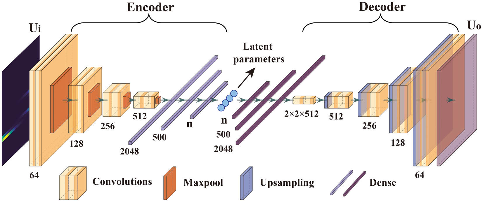
The network architecture used in this work is illustrated in Fig. 1, combining input layer Ui, convolutions, maxpool, fully connected layers, upsampling, and output layer Uo. The Ui and Uo in our model are the original spectral intensity and reconstructed spectral intensity, respectively. First, we fold the spectral intensity data of each round trip from 1024×1 to 32×32 and input Ui into the encoder layer. The encoder uses two-dimensional (2D) convolutional layers with kernels of 3×3, and the layers are 64,128, 256, and 512, respectively. Relu and 2×2 maxpool are used after each convolutional layer. Then, we straighten it into one-dimensional data of 2048 and connect the dense fully connected layers with 500 and n neurons, respectively, to obtain the latent parameter. Through the fully connected layer of n and 500, the one-dimensional data are transformed into 2×2×512 and then pass through the decoder. The decoder is symmetrical to the encoder, and the Relu activation function and 2×2 upsampling are used after each convolutional layer, while the final output Uo is 32×32. In order to evaluate the correlation between the output and ground truth, we calculate the cross-entropy loss function, H(y_,y)=−∑y_*lny,(2)where y_ and y represent the ground truth and output, respectively. Cross entropy represents the difference between two probability distributions, where the smaller the value, the closer the two distributions are.

For the case of double solitons collision, the system parameter is set as g0=2.4, r=2, ε=0.58, μ=−0.12, ν=0, β=0.1, Is=0.24, Γ=0.015 by using CQGLE. Under the condition that the system parameters remain unchanged, 10 groups of double solitons collision time-domain data are generated by changing the initial position of the pulse, as shown in Fig. 2. Different initial positions of solitons also affect the relative phase of solitons in the evolution process.

Double solitons undergo relative displacement under the influence of gain dynamics, resulting in collisions to form soliton molecules. The loss and recovery of the gain described by parameter Γ not only form the peak power difference between the front and back edge solitons, but also provide the attractive force between them. With the dynamic balance of the attractive force brought by the gain dynamics and the repulsive force of the spectral filtering, the soliton molecular structure with periodic oscillation is formed. We use Fourier technology to process the time-domain data to obtain the spectrum. Each group of spectral data is 10,000 × 1024, where 10,000 represents the number of round trips, and 1024 represents the number of points per round trip. The first nine groups of data have 90,000 round trips for training, and the last group of data has 10,000 round trips for testing.

The data set is normalized as the input of the constructed CAENN for training and testing. The Adam optimizer is used for training, and the learning rate is 0.0001. The batch size is 64 and the epoch number is 100. When the loss of 10 consecutive epoch tests does not change, the learning rate will be changed to one-tenth of the original. By changing the number n of neurons in the dense layer, it is found that the lowest training loss is 0.0511, and the validation loss is 0.0511.

The reconstructed data Uo is reverse-folded and spliced for each circle to recover the complete spectrum, as shown in Fig. 3(a). We find Pearson correlation coefficients (PCCs) with each round trip of the original spectrum; the results are shown in Fig. 3(b). PCC is used to reflect the degree of correlation between two variables. PCC (R) is calculated as follows: R=∑i=1n(Xi−X¯)(Yi−Y¯)∑i=1n(Xi−X¯)2∑i=1n(Yi−Y¯)2.(3)

For each round trip of spectral data, X represents the original spectral data, X¯ represents the mean value, Y represents the reconstructed spectral data, and Y¯ represents the mean value. The range of R is (−1, 1), and the greater the absolute value, the stronger the correlation. The average PCC between the reconstructed spectrum and the initial spectrum is 0.9989, which shows that CAENN can effectively reduce the dimension of the collision dynamics. Fourier transform is performed on each round trip of the reconstructed spectral data, and the filed autocorrelation trajectory is obtained, as shown in Fig. 3(c). CAENN reconstructs the double soliton collision dynamics under gain dynamics, including the relative displacement of solitons and oscillation dynamics. We compare the double soliton separation and the relative phase of the reconstructed 6000th round-trip data with the original data, as shown in Figs. 3(d) and 3(e). The relative phase and separation between the two solitons in the field autocorrelation trajectory are basically consistent with the original data, showing that the extracted features contain the basic information of interaction.

As shown in Fig. 4(a), when the reconstruction effect is the best, dense n is at least 3. By extracting the latent parameter, we find that the output of one column is 0 in Fig. 4(b), which means that the number of effective neurons is 2, consistent with the degrees of freedom in double soliton collision, namely, the separation and relative phase between double solitons.

For the case of triple solitons collision, the system parameter is set as g0=2.5, r=2, ε=0.58, μ=−0.12, ν=0, β=0.5, Is=0.32, Γ=0.002 by using CQGLE. Under the condition that the system parameters remain unchanged, by changing the initial position of the pulses, 10 groups of data of collision dynamics between triple solitons are generated with different relative phases; the typical collision dynamics is shown in Fig. 5. We also classify the dynamics data, where the first nine groups with 90,000 round trips spectral data are for training, and the last 10,000 round trips are for testing.

Similar to double solitons, the data set is normalized and put into the CAENN for training and testing. The training parameters are the same as those of double solitons, but the number n of neurons in the dense layer is different. Compared with the collision dynamics between two solitons, there is one more pulse in the triple soliton collision, so the process will be more complex and include a higher degree of freedom. By changing the number n of neurons in the dense layer, it is found that the lowest training loss is 0.0329, and the validation loss is 0.0328.

The reconstructed spectra are shown in Fig. 6(a), and the PCC with each round trip of the original spectrum is shown in Fig. 6(b). The average PCC between the reconstructed spectrum and the original spectrum is 0.9987. Compared with the results of double soliton collision, the decrease of similarity stems from the increase of system complexity. Figure 6(c) shows the field autocorrelation trajectory. The reconstructed field autocorrelation trajectory also includes the relative displacement of solitons and oscillation dynamics. Figures 6(d) and 6(e), respectively, show the reconstructed field autocorrelation trajectory and the original field autocorrelation trajectory in the 1680th round trip. The reconstructed spectrum can still accurately reproduce the basic parameters of soliton interaction.

As shown in Fig. 7, when the reconstruction effect is the best, dense number n is at least 4, consistent with the number of interaction parameters in triple soliton collision, i.e., the independent relative phase and separation among three solitons. The feature extraction of dynamics is based on the basic dimension of interaction. It shows that CAENN realizes the automatic coarsening of dynamic data by expressing the nonlinear structure of pulses with the neural network. CAENN can realize the minimum potential representation of soliton collisions without giving physical concepts. This representation is related to the number of independent dimensions of the physical system.

In conclusion, we have achieved effective data dimensionality reduction for double solitons and triple solitons collision dynamics based on CAENN, in which the average similarity between the reconstructed spectra and the original spectra is more than 99%. We found that the minimum number of latent parameters is consistent with the number of soliton interaction parameters, indicating that the autocoding of dynamics is based on the degrees of freedom of soliton interactions. This work will further promote the study of data dimensionality reduction of higher dimensional soliton dynamics in complex systems, such as spatiotemporal mode-locked fiber lasers. The feature extraction of pulse dynamics based on CAENN not only helps to greatly optimize the efficiency of laser self-tuning, but also provides new insights into the law of soliton interaction.

References

[1] D. R. Solli, B. Jalali. Analog optical computing. Nat. Photonics, 9, 704(2015).
[2] P. Grelu, N. Akhmediev. Dissipative solitons for mode-locked lasers. Nat. Photonics, 6, 84(2012).
[3] R. Weill, A. Bekker, V. Smulakovsky, B. Fischer, O. Gat. Noise-mediated Casimir-like pulse interaction mechanism in lasers. Optica, 3, 189(2016).
[4] E. Ding, S. Lefrancois, J. N. Kutz, F. W. Wise. Scaling fiber lasers to large mode area: an investigation of passive mode-locking using a multi-mode fiber. IEEE J. Quantum Electron., 47, 597(2011).
[5] K. J. Zhao, C. X. Gao, X. S. Xiao, C. X. Yang. Real-time collision dynamics of vector solitons in a fiber laser. Photonics Res., 9, 289(2021).
[6] J. He, P. Wang, R. He, C. Liu, M. Zhou, Y. Liu, Y. Yue, B. Liu, D. Xing, K. Zhu, K. Chang, Z. Wang. Elastic and inelastic collision dynamics between soliton molecules and a single soliton. Opt. Express, 30, 14218(2022).
[7] J. S. Peng, H. P. Zeng. Build-up of dissipative optical soliton molecules via diverse soliton interactions. Laser Photonics Rev., 12, 1800009(2018).
[8] X. M. Liu, X. K. Yao, Y. D. Cui. Real-time observation of the buildup of soliton molecules. Phys. Rev. Lett., 121, 023905(2018).
[9] Y. Q. Du, C. Zeng, Z. W. He, Q. Gao, D. Mao. Coherent dissipative soliton intermittency in ultrafast fiber lasers. Chin. Opt. Lett., 20, 011401(2022).
[10] M. Suzuki, O. Boyraz, H. Asghari, P. Trinh, H. Kuroda, B. Jalali. Spectral periodicity in soliton explosions on a broadband mode-locked Yb fiber laser using time-stretch spectroscopy. Opt. Lett., 43, 1862(2018).
[11] L. Salmela, N. Tsipinakis, A. Foi, C. Billet, J. M. Dudley, G. Genty. Predicting ultrafast nonlinear dynamics in fibre optics with a recurrent neural network. Nat. Mach. Intell., 3, 344(2021).
[12] M. Narhi, L. Salmela, J. Toivonen, C. Billet, J. M. Dudley, G. Genty. Machine learning analysis of extreme events in optical fibre modulation instability. Nat. Commun., 9, 4923(2018).
[13] T. Zahavy, A. Dikopoltsev, D. Moss, G. I. Haham, O. Cohen, S. Mannor, M. Segev. Deep learning reconstruction of ultrashort pulses. Optica, 5, 666(2018).
[14] J. Y. He, C. Y. Li, P. Wang, C. C. Liu, Y. G. Liu, B. Liu, D. K. Xing, Z. Wang. soliton molecule dynamics evolution prediction based on LSTM neural networks. IEEE Photon. Technol. Lett., 34, 193(2022).
[15] P. Y. Lu, S. Kim, M. Soljacic. Extracting interpretable physical parameters from spatiotemporal systems using unsupervised learning. Phys. Rev. X, 10, 031056(2020).
[16] R. Guidotti, A. Monreale, S. Ruggieri, F. Turin, F. Giannotti, D. Pedreschi. A survey of methods for explaining black box models. ACM Comput. Surv., 51, 1(2019).
[17] G. Genty, L. Salmela, J. M. Dudley, D. Brunner, A. Kokhanovskiy, S. Kobtsev, S. K. Turitsyn. Machine learning and applications in ultrafast photonics. Nat. Photonics, 15, 91(2021).
[18] X. Wei, J. C. Jing, Y. Shen, L. V. Wang. Harnessing a multi-dimensional fibre laser using genetic wavefront shaping. Light Sci. Appl., 9, 149(2020).
[19] G. Pu, L. Yi, L. Zhang, C. Luo, Z. Li, W. Hu. Intelligent control of mode-locked femtosecond pulses by time-stretch-assisted real-time spectral analysis. Light Sci. Appl., 9, 13(2020).
[20] A. J. Linot, M. D. Graham. Deep learning to discover and predict dynamics on an inertial manifold. Phys. Rev. E, 101, 062209(2020).
[21] C. Y. Li, J. Y. He, R. J. He, Y. E. Liu, Y. Yue, W. W. Liu, L. H. Zhang, L. F. Zhu, M. J. Zhou, K. Y. Zhu, Z. Wang. Analysis of real-time spectral interference using a deep neural network to reconstruct multi-soliton dynamics in mode-locked lasers. APL Photonics, 5, 116101(2020).
[22] G. E. Hinton, R. R. Salakhutdinov. Reducing the dimensionality of data with neural networks. Science, 313, 504(2006).
[23] R. Iten, T. Metger, H. Wilming, L. del Rio. Discovering physical concepts with neural networks. Phys. Rev. Lett., 124, 010508(2020).
[24] X. Ding, H. Chate, P. Cvitanovic, E. Siminos, K. A. Takeuchi. Estimating the dimension of an inertial manifold from unstable periodic orbits. Phys. Rev. Lett., 117, 024101(2016).
[25] M. Raissi, G. E. Karniadakis. Hidden physics models: machine learning of nonlinear partial differential equations. J. Comput. Phys., 357, 125(2018).
[26] B. Lusch, J. N. Kutz, S. L. Brunton. Deep learning for universal linear embeddings of nonlinear dynamics. Nat. Commun., 9, 4950(2018).
[27] P. R. Vlachas, G. Arampatzis, C. Uhler, P. Koumoutsakos. Multiscale simulations of complex systems by learning their effective dynamics. Nat. Mach. Intell., 4, 359(2022).
[28] S. H. Rudy, S. L. Brunton, J. L. Proctor, J. N. Kutz. Data-driven discovery of partial differential equations. Sci. Adv., 3, e1602614(2017).
[29] R. He, J. He, C. Li, L. Zhang, L. Zhu, M. Zhou, K. Zhu, Y. Liu, Y. Yue, Z. Wang. Transition between optical turbulence and dissipative solitons in a complex Ginzburg-Landau equation with quasi-CW noise. Phys. Rev. A, 103, 043515(2021).
[30] M. J. Ablowitz, T. P. Horikis, S. D. Nixon. Soliton strings and interactions in mode-locked lasers. Opt. Commun., 282, 4127(2009).
[31] R. He, Z. Wang, Y. Liu, Z. Wang, H. Liang, S. Han, J. He. Dynamic evolution of pulsating solitons in a dissipative system with the gain saturation effect. Opt. Express, 26, 33116(2018).
Set citation alerts for the article
Please enter your email address
© Copyright 2018-2021 | Chinese Laser Press. All Rights Reserved 沪ICP备15018463号-20