
Shaohua Hu, Jing Zhang, Qun Liu, Linchangchun Bai, Xingwen Yi, Bo Xu, Kun Qiu. Impacts of the measurement equation modification of the adaptive Kalman filter on joint polarization and laser phase noise tracking[J]. Chinese Optics Letters, 2022, 20(2): 020603
- Chinese Optics Letters
- Vol. 20, Issue 2, 020603 (2022)
Abstract
1. Introduction
Polarization division multiplexing plays an important role to double the spectral efficiency for high speed coherent optical fiber transmissions. The polarization de-multiplexing algorithms can be divided into blind equalization and data-aided multi-input multi-output (MIMO) algorithms. The blind algorithms are mainly based on the characteristic of constellation points, such as constant modulus algorithm (CMA), multi-modulus algorithm (MMA), and cascaded MMA (CMMA), together with their variants[
The Kalman filtering (KF) has been widely used in system control, which has been introduced into optical communications in recent years. KF has both blind[
In this paper, we analyze the noise tolerance of CKF and MKF in theory by introducing conditional variance of measurement residual and process noise. We find that the enhanced noise tolerance of MKF compared with CKF results from the decrease of the mean square error in each iteration by numerical simulations. Besides, the covariance reduction indicates the noise tolerance improvement of MKF, which results in better tracking ability and covariance initialization flexibility. Furthermore, we find the noise covariance matching method can be smoothly combined with MKF to adaptively update the covariance matrices of measurement noise and process noise. We call it adaptive MKF corresponding to adaptive CKF. The simulation comparison between adaptive CKF and adaptive MKF is conducted in virtual photonics instrument (VPI)-MATLAB co-simulation on a single carrier quadrature amplitude modulation (QAM)-16 coherent optical fiber transmission system. Compared with adaptive CKF, adaptive MKF has optical SNR (OSNR) improvement at the scrambling rate of 10 MHz, and around 73.5% scrambling rate improvement at the OSNR of 24 dB. Particularly, the adaptive MKF retains the successful joint tracking of the fast RSOP and laser phase noise in the lower OSNR cases. For higher OSNR, either the MKF or adaptive MKF outperforms CKF or adaptive CKF in initialization flexibility.
Sign up for Chinese Optics Letters TOC. Get the latest issue of Chinese Optics Letters delivered right to you!Sign up now
2. Theoretical Comparisons between CKF and MKF
Before the comparison, we denote the channel model and variables of the transmission system. The polarization diversity multiplexing (PDM) coherent optical transmission is assumed to be linear and the discrete-time form of the received signal after dispersion compensation can be expressed as
The model of CKF and MKF is defined as follows. During the iteration process of KF, the convergence can be achieved by minimizing the difference between the predicted signal and the observed signal. It is assumed that and are signals predicted by CKF and MKF. In CKF, can be derived by
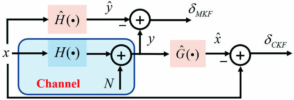
The difference in measurement residual between CKF and MKF is illustrated in Fig. 1. For CKF, the noisy terms and the predicted measurement are multiplied together to influence the measurement residual. While MKF differs from CKF, only one noise-related factor contributes to the prediction , and the two noisy terms and additively act on the measurement residual. We show the equalization model and state estimation process in Fig. 2.
![]()
Figure 1.Measurement residuals of CKF and MKF.
![]()
Figure 2.Equalization model and state estimation process of MKF.
Apart from the measurement residual, the KF algorithm also minimizes the process noise. and are defined as the state matrix of CKF and MKF, respectively. The process noises and in each iteration for CKF and MKF can be expressed in Eqs. (7) and (8):
To concentrate on the noise tolerance analysis of the two schemes, we degenerate the theoretical analysis into single polarization. Substituting in Eq. (5) with Eq. (7), we derive the measurement residual of CKF as
Similarly, we have the measurement residual ,
According to Eqs. (9) and (10), the process noise for CKF and MKF versus the measurement residual can be expressed as
We introduce the conditional variance of measurement residuals and process noises for CKF and MKF to evaluate the noise tolerance and to explore their interaction during each prediction and innovation iteration. We define the conditional variance of when sequence is transmitted as
Similarly, we have
To avoid the complicated analytical derivation in variance calculation, numerical simulations are conducted to compare the noise tolerance between CKF and MKF based on Eqs. (13)–(16), where a 16-QAM sequence with complex symbols is transmitted through the AWGN channel. For simplicity, we compare the process noises by setting the channel-scaling factor, , which leads to . Figures 3(a) and 3(b) show the conditional variance curves of measurement error and process noise varying with process noise and measurement error at different SNRs. To fully compare the conditional variance, we set the axis in logarithmic scale, which covers the cases with both slighter and stronger noise. We take specific values of two variables to illustrate the rationality of the abscissa of Figs. 3(a) and 3(b). Since the I- or Q-component of the transmitted QAM signal ranges from to 3, in Fig. 3(a) indicates that the measurement residual is on the same order of magnitude as the transmitted signal, which is large enough for a convergent Kalman filter. In Fig. 3(b), also provides the conditional variance under the situation with larger process noise. As shown in Figs. 3(a) and 3(b), both the conditional variances of process noise and measurement error for MKF are always smaller than those of CKF. The gaps between MKFs and CKFs occur in practical SNRs and tend to be more obvious for lower SNR cases.
![]()
Figure 3.(a) Variance of process noise versus the measurement error; (b) variance of measurement noise versus the process noise.
To compare the SNR robustness between MKF and CKF, we further depict the ratio of and versus SNRs at different process noise levels, as shown in Fig. 4. All of the conditional variance ratios are larger than one, which indicates that MKF always introduces a smaller measurement residual, especially for channels with higher noise power.
![]()
Figure 4.Variance rate of measurement errors versus SNR.
Therefore, for the general SNR region, we always have
Inequalities (19) and (20) also hold in all practical channel noise powers, as shown in Fig. 3, which indicates MKF outperforms CKF in noise tolerance, especially for large noise. This also explains the better noise tolerance for MKF compared with CKF in our previous experiment[
For stability and real implementation, we introduce the noise covariance matching method into MKF, since it has lower complexity and is more practical to implement than other adaptive algorithms[
When the channel is memorial, the state vector can be extended to multi-tap. When obtaining the multi-tap state vector , we can reshape the state vector to the channel response matrix and determine its pseudo-inverse matrix as if the columns of are linearly dependent. Besides, the inter-symbol interference can also be mitigated by conventional adaptive equalizers with the least mean squares (LMS) or recursive least squares (RLS) algorithms.
3. Simulation Comparisons of the Tracking Abilities
In this section, we conduct numerical simulations to testify the proposed modified adaptive Kalman filter for joint polarization and phase noise tracking. The simulation system is a conventional polarization-multiplexed coherent 16-QAM optical transmission system established in VPI 9.1. System parameters are shown in Table 1. The block of RSOP is set based on Eq. (2), where the angle varies in a sinusoidal form with the scrambling frequency . At the receiver, frequency-domain group velocity dispersion compensation, fourth power FFT-based frequency offset compensation, and match filter are applied before the Kalman filter. The adaptive KF is adopted for polarization de-multiplexing and phase recovery. Both CKF and MKF adopt the covariance matching adaptive algorithm with the initial covariance of 0.5.
| Parameter | Value |
|---|---|
| Baud rate | 28 GBaud |
| Pulse shaping | RRC |
| Training length | 100 |
| Signal linewidth | 100 kHz |
| PMD coefficient | |
| Dispersion | 16 ps/(nm·km) |
| Sampling rate | 112 GSa/s |
| Rolling factor | 0.1 |
| Freq. offset | 100 MHz |
| Fiber length | 400 km |
| Linewidth (LO) | 100 kHz |
Table 1. Simulation Parameter Setup
3.1. Noise tolerance
We first compare the tracking performance between adaptive CKF and adaptive MKF at different OSNRs, as shown in Fig. 5, where we also compare the performance of the extended CKF (ECKF) and pilot-aided averaging window method (AWM) as a reference, where the ECKF still regards the measurement variable as the transmitted symbols but estimates the Jones matrix and laser phase noise separately. The AWM inserts three pilot symbols between every 17 symbols and smooths the estimation noise by time averaging. The pilot overhead of AWM is 15%, while for KF the number of training symbols is 100. The overhead of KF is much less than AWM. The scrambling rate of RSOP is 10 MHz and 20 MHz, corresponding to Figs. 5(a) and 5(b), both of which have the linewidth of 100 kHz. The performances are evaluated at the 20% forward error correction (FEC) limit, i.e., the bit error rate (BER) of .
![]()
Figure 5.BER of the recovered signal versus OSNR. The scrambling rate is (a) 10 MHz and (b) 20 MHz. The reference curves (gray dashed lines) are under the back-to-back (B2B) case without RSOP.
When the OSNR is below 18 dB, the divergence of KF mainly results from the noise sensitivity of the second stage of Kalman filter. The BER performance of MKF and CKF mainly differs from each other within 18 to 24 dB since the noise tolerance of KF differs in this range. We find MKF outperforms CKF and ECKF for both cases and has OSNR improvement over CKF at the 20% FEC limit. When the scrambling rate increases to 20 MHz, 3.5 dB OSNR gain is observed compared with CKF, while 1.87 dB OSNR gain is observed compared with ECKF. AWM works better than KF at extremely low OSNRs, which benefits from its very large overhead. Once KF converges, the BERs rapidly drop below those of AWM.
3.2. Scrambling rate tolerance
We then compare the tracking ability of the adaptive CKF and MKF with lower and larger noise powers. Figures 6(a) and 6(b) show the BER performances for CKF and MKF versus scrambling rate at the OSNRs of 24 dB and 20 dB. The trends can be divided into three segments, i.e., the optimum stage (the scrambling rate is lower than 10 MHz), the transition stage (the scrambling rate from 20 MHz to 35 MHz at 24 dB OSNR, from 10 MHz to 20 MHz at 20 dB OSNR), and the divergence stage (the higher scrambling rate).
![]()
Figure 6.(a) Signal qualities versus scrambling rates at the OSNR of 24 dB; (b) signal qualities versus scrambling rates at the OSNR of 20 dB.
Focusing on the transition stage, i.e., the extreme tracking performance for CKF and MKF, we find that CKF and ECKF diverge sharply at the OSNR of 24 dB, whereas the performance of MKF deteriorates gradually. From Fig. 6(a), we find that MKF can converge under the scrambling rate up to 35 MHz, around 73.5% enhancement over CKF, i.e., 14.83 MHz. When the OSNR is 20 dB, CKF diverges, but MKF still has scrambling rate tolerance, as shown in Fig. 6(b). This is because the enhanced channel noise has higher probability to induce cycle-slip or algorithm divergence.
At the optimum stage for the OSNR of 24 dB, the CKF and MKF have similar performances. For the OSNR of 20 dB, MKF can tolerate higher scrambling rate than ECKF at 20% FEC limit, while CKF fails to track the fast RSOP in the megahertz (MHz) level. MKF and ECKF outperform AWM in both cases, even though MKF is a kind of linear KF. The results are consistent with Fig. 5, which shows that MKF can work stably in relatively lower OSNR.
3.3. Parameter initialization flexibility
Finally, we investigate the parameter initialization tolerance with and without the Q/R adaptive algorithm. We show the BERs versus the initial Q and R with hot maps in Fig. 7, where the OSNR is 30 dB. In Fig. 7, the required R is proportional to but larger than Q when the Q/R adaptive algorithm is not enabled. Comparing the BER performance of MKF with CKF, we find MKF outperforms CKF, as shown in the blue regions of the hot maps in Figs. 7(a) and 7(c), which indicates a higher flexibility of MKF in Q/R initialization that is mainly brought from the improved noise tolerance of MKF.
![]()
Figure 7.Initialization tolerance of Q/R parameter for linear CKF and MKF at the OSNR of 30 dB and 10 MHz scrambling rate. (a) CKF without Q/R adaptive algorithm; (b) CKF with Q/R adaptive algorithm; (c) MKF without Q/R adaptive algorithm; (d) MKF with Q/R adaptive algorithm.
When the adaptive algorithm is applied to the Kalman filters, the convergence regions are only dependent on the initial R. We find that the Q/R adaptive algorithm can also effectively improve the flexibility of MKF, since both the convergence regions of CKF and MKF are expanded significantly. This indicates that the adaptive algorithm can improve the robustness of MKF at higher OSNRs. While for lower OSNRs, adaptive MKF succeeds in tracking the fast RSOP but adaptive CKF fails, as discussed in Section 3.2.
The simulation results in Section 3 are concluded in Table 2 for a clear comparison. Based on the discussion above, our findings are as follows. (1) MKF has higher noise tolerance than CKF especially with lower OSNRs. (2) The modification improves the tracking speed and initialization flexibility, which benefits from the improved noise tolerance. (3) The noise covariance matching approach is effective for improving the initialization flexibility of MKF.
| Filter Type | Min. OSNR at 10 MHz RSOP (dB) | Max. RSOP at 24 dB OSNR (MHz) | Max. RSOP at 20 dB OSNR (MHz) | Initialization Tolerance without Adaptive Algorithm |
|---|---|---|---|---|
| CKF | 22 | 22 | Worse | |
| MKF | 19 | 37 | 20 | Better |
Table 2. Performance Comparison for Kalman Filters
4. Conclusions
Both theoretical analysis and simulation results have shown that the MKF has higher robustness to noise-induced decision error and covariance matrices initialization that are related to the tracking ability in the presence of fast RSOP. Higher tracking speed (up to 50% improvement from CKF), better OSNR tolerance ( improvement from CKF), and superior initialization flexibility are observed from MKF. The MKF combined with the covariance matching method outperforms the adaptive CKF, especially in the case of lower OSNR.
References
[1] J. Zhang, J. Yu, N. Chi, H.-C. Chien. Time-domain digital pre-equalization for band-limited signals based on receiver-side adaptive equalizers. Opt. Express, 22, 20515(2014).
[2] X. Zhou, K. Zhong, J. Huo, L. Gao, Y. Wang, L. Wang, Y. Yang, J. Yuan, K. Long, L. Zeng, A. P. T. Lau, C. Lu. 112 Gb/s transmission over 80 km SSMF using PDM-PAM4 and coherent detection without optical amplifier. Opt. Express, 24, 17359(2016).
[3] C. Zhu, A. V. Tran, S. Chen, L. B. Du, T. Anderson, A. J. Lowery, E. Skafidas. Improved two-stage equalization for coherent Pol-Mux QPSK and 16-QAM systems. Opt. Express, 20, B141(2012).
[4] P. Johannisson, M. Sjödin, M. Karlsson. A modified CMA for PS-QPSK. Signal Processing in Photonic Communications, SPTuB3(2011).
[5] L. Lu, Y. Lei, J. Lei, X. Zou, W. Sheng. Analysis of singularity problem from CMA induced by PDL in polarization demultiplexing. Asia Communications and Photonics Conference, AF2F.40(2013).
[6] P. Johannisson, H. Wymeersch, M. Sjödin, A. S. Tan, E. Agrell, P. A. Andrekson, M. Karlsson. Convergence comparison of the CMA and ICA for blind polarization demultiplexing. J. Opt. Commun. Netw., 3, 493(2011).
[7] X. Li, W.-D. Zhong, A. Alphones, C. Yu, Z. Xu. Channel equalization in optical OFDM systems using independent component analysis. J. Lightwave Technol., 32, 3206(2014).
[8] H. Zhang, Z. Tao, L. Liu, S. Oda, T. Hoshida, J. C. Rasmussen. Polarization demultiplexing based on independent component analysis in optical coherent receivers. 34th European Conference on Optical Communication, 1(2008).
[9] N. Nabavi, T. J. Hall. Demultiplexing by independent component analysis in coherent optical transmission: the polarization channel alignment problem. 2015 Photonics North, 1(2015).
[10] P. M. Krummrich, D. Ronnenberg, W. Schairer, D. Wienold, F. Jenau, M. Herrmann. Demanding response time requirements on coherent receivers due to fast polarization rotations caused by lightning events. Opt. Express, 24, 12442(2016).
[11] Q. Xiang, Y. Yang, J. Cao, Q. Zhang, Y. Yao. Polarization tracking for Stokes-vector modulation formats using Kalman filter. CLEO Pacific Rim Conference, W3A.19(2018).
[12] Z. Zheng, N. Cui, H. Xu, X. Zhang, W. Zhang, L. Xi, Y. Fang, L. Li. Window-split structured frequency domain Kalman equalization scheme for large PMD and ultra-fast RSOP in an optical coherent PDM-QPSK system. Opt. Express, 26, 7211(2018).
[13] T. Marshall, B. Szafraniec, B. Nebendahl. Kalman filter carrier and polarization-state tracking. Opt. Lett., 35, 2203(2010).
[14] N. Cui, Z. Zheng, X. Zhang, W. Yi, R. Guo, W. Zhang, X. Tang, H. Xu, L. Xi. Joint blind equalization of CD and RSOP using a time-frequency domain Kalman filter structure in Stokes vector direct detection system. Opt. Express, 27, 11557(2019).
[15] W. Yi, Z. Zheng, N. Cui, X. Zhang, L. Qiu, N. Zhang, L. Xi, W. Zhang, X. Tang. Joint equalization scheme of ultra-fast RSOP and large PMD compensation in presence of residual chromatic dispersion. Opt. Express, 27, 21896(2019).
[16] N. Cui, X. Zhang, Z. Zheng, H. Xu, W. Zhang, X. Tang, L. Xi, Y. Fang, L. Li. Two-parameter-SOP and three-parameter-RSOP fiber channels: problem and solution for polarization demultiplexing using Stokes space. Opt. Express, 26, 21170(2018).
[17] B. Wang, Z. Li. Uniformly high-speed semi-open loop polarization control and PMD suppression. Chin. Opt. Lett., 18, 050601(2020).
[18] S. Wang, Z. Li. Polarization scrambling characteristic analysis based on density of polarization states statistics. Chin. Opt. Lett., 18, 060604(2020).
[19] Y. Jiang, X. Yi, S. Hu, X. Huang, W. Tang, W. Zhou, X. Huang, J. Zhang, K. Qiu. Polarization de-multiplexing using a modified Kalman filter in CO-OFDM transmissions. Chin. Opt. Lett., 17, 030603(2019).
[20] Q. Zhang, Y. Yang, Q. Xiang, Q. He, Z. Zhou, Y. Yao. Noise adaptive Kalman filter for joint polarization tracking and channel equalization using cascaded covariance matching. IEEE Photonics J., 10, 7900911(2018).
[21] N. Cui, X. Zhang. Fast tracking of polarization impairments using DSP algorithms in fiber for a coherent optical communication system. Microwave Opt. Technol. Lett., 63, 2453(2021).

Set citation alerts for the article
Please enter your email address
© Copyright 2018-2021 | Chinese Laser Press. All Rights Reserved 沪ICP备15018463号-20