Discrepancy between transmission spectrum splitting and eigenvalue splitting: a reexamination on exceptional point-based sensors

Qi Geng; Ka-Di Zhu

doi:10.1364/PRJ.423996

Abstract

In the study of exceptional point (EP)-based sensors, the concrete form of the output spectrum is often dismissed, and it is assumed that there is a corresponding relation between the peaks/valleys in the transmission spectrum and the real parts of the eigenvalues of the system. We point out that this assumption does not always hold. An effect, which is mathematically similar to electromagnetically induced transparency (EIT), may result in a ‘pseudo spectrum splitting’ that does not correspond to the splitting between the eigenvalues. The effect shall be taken care of when designing an EP-based sensor since it may cause measurement error and misunderstanding such as recognization of the spectrum splitting as the eigenvalue splitting at the exceptional point. We also propose to intentionally utilize this ‘pseudo splitting’ to design a sensor, which does not work at an EP, that has an EP-like spectrum splitting.

1. INTRODUCTION

A peculiar kind of degeneracy is known as the exceptional point (EP) [1 –4]. At an EP, not only the eigenvalues, but also the eigenvectors coalesce. A small perturbation ( $ϵ$ ) exerted on an $N$ -fold EP will result in a eigenvalue splitting that is proportional to $ϵ^{1 / N}$ , while for a non-exceptional degeneracy known as the diabolic point (DP), the eigenvalue splitting is proportional to $ϵ$ . Based on the fact that for a small $ϵ$ the EP kind of splitting is larger, EP-based sensors [5,6] have been proposed for high precision measurement. The EP is often realized in optical systems [7], and two typical realizations of an optical EP are a microdisk with scatters [5,8,9] and coupled optical cavities [10 –12].

Most theoretical studies on the optical EP do not concern with the concrete form of the output spectrum. They devoted to the structure of the eigenvalues of the system’s Hamiltonian, and make a simple assumption that the peaks/valleys of the spectrum correspond to the real parts of the Hamiltonian’s eigenvalues, the linewidths of the peaks/valleys correspond to the imaginary parts of the eigenvalues, and the splitting of the peaks/valleys can only be discerned if the splitting is large compared with the linewidths. The central point of this paper is to show that the above assumption is not exact, and the inexactness may affect the validity or precision of some EP-based sensing schemes that is based on the valleys in the transmission spectrum.

In fact, electromagnetically induced transparency (EIT) [13] is a typical case that invalidates the correspondence relation between transmission spectrum splitting and eigenvalue splitting. EIT was initially proposed by Harris and co-workers in a three-level $Λ$ -type atomic system [14]: by applying a strong coupling field between a metastable state and the upper state of an allowed transition to ground, one may obtain a resonantly enhanced third-order susceptibility while at the same time inducing transparency of the media. The notion has been generalized to and has been studied in atomic and molecular systems, superconductors, optomechanics, whispering-gallery mode microcavities (WGMRs), and so on (see Ref. [15], Fig. 1, and Table 1). The point is, while the transparency window in EIT is reminiscent of eigenvalue splitting and in the strong coupling regime the transparency window fits well with the eigenvalue splitting [15], in many cases the transparency window and the eigenvalue splitting do not coincide. In particular, in the weak coupling regime, there can be no eigenvalue splitting while the transparency window still exists.

Sign up for Photonics Research TOC. Get the latest issue of Photonics Research delivered right to you！Sign up now

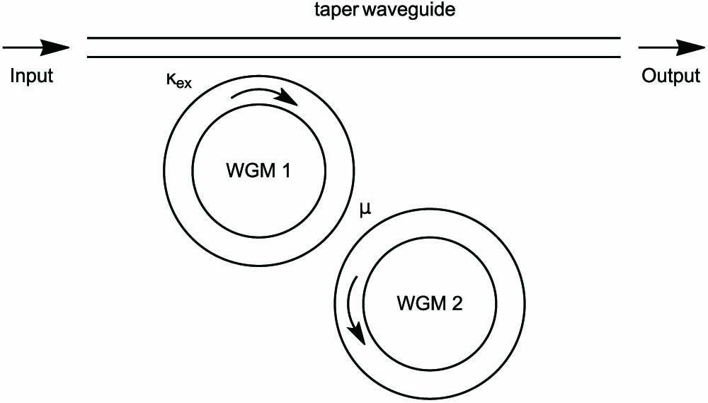
Schematic of the system consisting of two coupled whispering-gallery microcavities. We have not explicitly drawn the taper in the figure.

Figure 1.Schematic of the system consisting of two coupled whispering-gallery microcavities. We have not explicitly drawn the taper in the figure.

In this paper, we express the output spectrum of two coupled WGMRs as the ratio of two polynomials. The polynomial in the denominator is the characteristic polynomial $C (w)$ of the effective Hamiltonian’s eigenvalues, while the polynomial in the numerator, $P (w)$ , is another second-order polynomial. The point is, while the eigenvalues of the system are related to $C (w)$ , $C (w)$ and $P (w)$ together determine the valleys in the spectrum. In fact, in most cases, the valleys correspond to the roots of $P (w) = 0$ , in contrast to the common knowledge that the valleys in the spectrum correspond to the roots of $C (w) = 0$ (i.e., eigenvalues). This discrepancy between eigenvalues and the valleys in the spectrum may cause confusion, making people wrongly recognize the valleys in the spectrum as the eigenvalues of the system. Since these “fake valleys” appear when the two valleys are close, the caution shall be taken when explaining the spectrum splittings in the experiments as the eigenvalue splittings at EPs. We also note that a by-product of our formulation is to provide a unified and transparent description of EIT and spectrum splitting caused by eigenvalue splitting.

In a word, we suggest that there is a flaw in existing theory of EP-based sensors: the valleys in the transmission spectrum may not correspond to the real parts of the eigenvalues. We can even conversely utilize the above fact to construct a sensing scheme that does not correspond to an EP, while showing an EP-like spectrum splitting. We show this in Section 4.

This paper is organized as follows. In Section 2, we derive the expression of the output spectrum of two coupled WGMRs. The method can be generalized to generic two-mode systems without difficulty. In Section 3, we illustrate the discrepancy between the valleys in the spectrum and the eigenvalues of the Hamiltonian. We discuss, respectively, the case $w_{1} = w_{2}$ and $w_{1} \neq w_{2}$ in each subsection. In Section 4, we show that the above discrepancy can be conversely utilized to design high precision sensors, which do not work at the EPs, that exhibit EP-like, square root proportional spectrum splittings.

2. OUTPUT SPECTRUM OF TWO COUPLED WHISPERING-GALLERY MICROCAVITIES

We illustrate our idea based on coupled optical cavities (e.g., coupled whispering-gallery microcavities [12]), as shown in Fig. 1. The effective Hamiltonian of two coupled WGMs features that the off-diagonal elements are mutually complex conjugated (without loss of generality, we choose them to be the same real value $μ$ ). The feature is shared by most two-mode linear optical systems, while there are cases that the off-diagonal elements are asymmetric, e.g., for a microdisk with scatters [5,8,9], there is no difficulty to apply the method to these systems.

In a two-mode approximation, the Hamiltonian of the system of two coupled WGMs, without the input and the noise taken into account, can be represented by a $2 \times 2$ matrix: $H = ℏ (\begin{matrix} w_{1} - i \frac{κ_{1}}{2} & μ \\ μ & w_{2} - i \frac{κ_{2}}{2} \end{matrix}) .$ (1)

We use $a_{1}$ and $a_{2}$ to denote the amplitudes of the two modes. $w_{1}$ is the resonant frequency of the first whispering-gallery microcavity, while $w_{2}$ is the resonant frequency of the second whispering-gallery microcavity. $κ_{1}$ and $κ_{2}$ are the overall cavity intensity decay rates for microcavity 1 and microcavity 2, respectively. The equation of motion, with an input $a_{in}$ injected into cavity 1, is $\frac{d}{d t} (\begin{matrix} a_{1} \\ a_{2} \end{matrix}) = - i (\begin{matrix} w_{1} - i \frac{κ_{1}}{2} & μ \\ μ & w_{2} - i \frac{κ_{2}}{2} \end{matrix}) (\begin{matrix} a_{1} \\ a_{2} \end{matrix}) + (\begin{matrix} \sqrt{κ_{ex}} a_{in} \\ 0 \end{matrix}),$ (2)in which $κ_{ex}$ refers to the loss rate associated with the input coupling [16]. We note that $k_{1} = κ_{01} + κ_{ex}$ , in which $κ_{01}$ refers to the loss aside from the input port. We have used a classical (in contrast to quantum) approach and have neglected the noise term. The classical approach is sufficient for our purpose since we aim to point out the defect of the former understanding, which is as well based on a classical approach.

Equation (2) can be rewritten in the frequency domain as $- i (\begin{matrix} w - w_{1} + i \frac{κ_{1}}{2} & - μ \\ - μ & w - w_{2} + i \frac{κ_{2}}{2} \end{matrix}) (\begin{matrix} a_{1} (w) \\ a_{2} (w) \end{matrix}) = (\begin{matrix} \sqrt{κ_{ex}} a_{in} (w) \\ 0 \end{matrix}),$ (3)and via using the Cramer’s rule, the solution of the amplitude of the first cavity can be derived as $a_{1} (w) = \frac{i \sqrt{κ_{ex}} (w - w_{2} + i \frac{κ_{2}}{2})}{| \begin{matrix} w - w_{1} + i \frac{κ_{1}}{2} & - μ \\ - μ & w - w_{2} + i \frac{κ_{2}}{2} \end{matrix} |} a_{in} (w),$ (4)in which the determinant in the denominator is the characteristic polynomial of $H$ . The solution can be rewritten as $a_{1} (w) = \frac{i \sqrt{κ_{ex}} (w - w_{2} + i \frac{κ_{2}}{2})}{(w - λ_{1}) (w - λ_{2})} a_{in} (w),$ (5)in which $λ_{1}$ and $λ_{2}$ are the eigenvalues of the Hamiltonian $H$ .

The output spectrum, according to the input-output relation [16], is $a_{out} = a_{in} - \sqrt{κ_{ex}} a_{1} .$ (6)

Thus, the output spectrum can be written as $a_{out} (w) = \frac{P (w)}{(w - λ_{1}) (w - λ_{2})} a_{in},$ (7)in which $P (w)$ is a second-order polynomial: $P (w) = (w - λ_{1}) (w - λ_{2}) - i κ_{ex} (w - w_{2} + i \frac{κ_{2}}{2}) .$ (8)

The transmission rate can be rewritten as $T = {| \frac{(w - r_{1}) (w - r_{2})}{(w - λ_{1}) (w - λ_{2})} |}^{2},$ (9)in which $r_{1}$ and $r_{2}$ are the roots of $P (w) = 0$ . We can see from Eq. (9) that, roughly, $T$ obtains its minimum near $r_{1,2}$ . This is in contrast to the intuition (misunderstanding) that the minimum is obtained at the eigenvalues, i.e., $λ_{1,2}$ . The misunderstanding results from several factors, and the main factor is that for a large $μ$ , the roots of $P (w)$ approach $λ_{1}$ and $λ_{2}$ , which lets us think that the valleys in the spectrum correspond to the eigenvalues of the system.

In a more strict sense, $T$ may not obtain its minimum at or near $Re (r_{1,2})$ . If the imaginary part of $r_{1} (r_{2})$ is comparable with the corresponding eigenvalue’s imaginary part, then the minimum may be obtained neither near $r_{1} (r_{2})$ nor $λ_{1} (λ_{2})$ . On the other hand, if the imaginary part of $r_{1} (r_{2})$ is much smaller than the imaginary part of $λ_{1} (λ_{2})$ as well as the real splitting between $r_{1}$ and $r_{2}$ , then we can assert that $T$ obtains its minimum at $r_{1} (r_{2})$ . This is the case if the system is in critical coupling $κ_{ex} = κ_{1} / 2$ and $κ_{1} ≫ κ_{2}$ , which is a common case in EIT. In Section 3, we choose such a case for discussion.

3. DISCREPANCY BETWEEN THE TRANSMISSION VALLEYS AND THE EIGENVALUES

In this section, we follow the above formulas, substitute a set of concrete parameters, and show the discrepancy between the transmission valleys and the eigenvalues explicitly.

A. Case of $w_{1} = w_{2}$

We pick the parameters to be $w_{1} = w_{2} = 10 GHz$ , $κ_{1} / 2 = 1 MHz$ , $κ_{2} / 2 = 0.1 MHz$ , and $κ_{ex} = κ_{1} / 2$ . The last condition refers to the situation of “critical coupling” [16], for which the output on resonance and without coupling is zero. We have intentionally choose $κ_{1} ≫ κ_{2}$ , which resembles to the case in EIT [15].

In Fig. 2, we plot the transmission rates for $μ = 0$ , $μ = 0.2 MHz$ , and $μ = 0.5 MHz$ . The corresponding eigenvalues of the system are $λ_{1} = 10, 000 - 0.15 i MHz$ , $λ_{2} = 10, 000 - 0.95 i MHz$ for $μ = 0.2 MHz$ , and $λ_{1} = 9999.78 - 0.55 i MHz$ , $λ_{2} = 10, 000.22 - 0.55 i MHz$ for $μ = 0.5 MHz$ . We can see from Fig. 2 that the valleys in the spectrum do not correspond to the eigenvalues of the Hamiltonian. For $μ = 0.2 MHz$ , there is no splitting in the real parts of the eigenvalues; however, a splitting in the spectrum appears. This splitting coincides with the roots of $P (w) = 0$ . For $μ = 0.5 MHz$ , the minimum points agree with the roots of $P (w) = 0$ , while they do not agree with the eigenvalues of the system.

Figure 2.Spectrum of two coupled cavities, which has a splitting similar to EIT. The parameters are $w_{1} = w_{2} = 10 GHz$ , $κ_{1} / 2 = 1 MHz$ , $κ_{2} / 2 = 0.1 MHz$ , $κ_{ex} = κ_{1} / 2$ , and $μ = 0, 0.2, 0.5 MHz$ . The corresponding eigenvalues as well as the roots of $P (w) = 0$ are as follows: for $μ = 0$ , $λ_{1} = 10, 000 - i$ , $λ_{2} = 10, 000 - 0.1 i$ , $r_{1} = 10, 000$ , $r_{2} = 10, 000 - 0.1 i$ ; for $μ = 0.2 M H z$ , $λ_{1} = 10, 000 - 0.15 i$ , $λ_{2} = 10, 000 - 0.95 i$ , $r_{1} = 9999.81 - 0.05 i$ , $r_{2} = 10, 000.19 - 0.05 i$ ; for $μ = 0.5 MHz$ , $λ_{1} = 9999.78 - 0.55 i$ , $λ_{2} = 10, 000.22 - 0.55 i$ , $r_{1} = 9999.50 - 0.05 i$ , $r_{2} = 10, 000.50 - 0.05 i$ .

In Fig. 3, we plot the difference of the real parts of the eigenvalues, the difference of the real parts of the roots of $P (w) = 0$ , and the splitting width in the transmission spectrum with different $μ$ . We see from the figure that the splitting of the eigenvalues of the system does not correspond to the valleys in the spectrum. It is the splitting of the roots of $P (w) = 0$ , instead, that indicates the splitting width of the transmission spectrum. With $μ$ increasing, $Re (Δ λ)$ approaches $Re (Δ r)$ and, thus, agrees with the splitting width in the transmission spectrum.

Figure 3. $Re (Δ λ)$ denotes the real splitting between the eigenvalues, $Re (Δ r)$ denotes the real splitting between the roots of $P (w) = 0$ , and $Δ W$ denotes the splitting in the spectrum. $Δ W$ agrees with $Re (Δ r)$ . When $μ$ is large, $Re (Δ λ) \approx Re (Δ r)$ . The parameters are the same as in Fig. 2.

We can see from Fig. 3 that the splitting width equals $Re (Δ r)$ for a wide range of $μ$ . While the fact is well known in case the coupling is strong, i.e., $μ > κ_{1} / 2$ , it may not so familiar that two well-resolved valleys with the splitting width can appear for $μ ≪ κ_{1}$ .

B. Case of $w_{1} \neq w_{2}$

The parameters in Fig. 4 are $w_{1} = 10, 000 MHz$ , $w_{2} = 10, 000.1 MHz$ , $κ_{1} / 2 = 1 MHz$ , $κ_{2} / 2 = 0.1 MHz$ , and $μ = 0.3 MHz$ . As shown in Fig. 4, there would be a large error if we recognize the valleys in the spectrum as the eigenvalues of the Hamiltonian.

Figure 4.Transmission rate in case $w_{1} \neq w_{2}$ . There is a large discrepancy between the eigenvalues of the system and the valleys in the spectrum. The parameters are $w_{1} = 10, 000 MHz$ , $w_{2} = 10, 000.1 MHz$ , $κ_{1} / 2 = 1 MHz$ , $κ_{2} / 2 = 0.1 MHz$ , and $μ = 0.3 MHz$ .

We suggest that this discrepancy shall be taken care of when designing an EP-based sensor, especially for the sensing schemes aimed to detect the small variation in a diagonal element in the Hamiltonian.

4. CONSTRUCTING AN EP-LIKE SPECTRUM SPLITTING

In this section, we intentionally use the above discrepancy to construct a sensing scheme. The scheme exhibits EP-like spectrum splittings (proportional to the square root of the perturbations), though it does not work at an EP. The sensing scheme also shows a violation to the understanding that, to observe a perturbation induced spectrum splitting, the imaginary parts of the eigenvalues will be small compared to the splitting, which is well accepted in previous studies of sensors based on spectrum splittings. The central idea of our scheme is to construct a $P (w)$ , which has repeated real roots. This can be achieved by using an overcoupled cavity with $κ_{ex} = κ_{1} / 2 + κ_{2} / 2$ , and setting the base coupling coefficient to be $μ_{0} = κ_{2} / 2$ .

We choose the parameters to be $w_{1} = w_{2} = 10 GHz$ , $κ_{1} / 2 = κ_{2} / 2 = κ_{ex} / 2 = 1 MHz$ , $μ_{0} = 1 MHz$ , and $μ = μ_{0} + Δ μ$ . We see from Fig. 5 that a perturbation $Δ μ = 0.1 MHz$ results in a spectrum splitting $\approx 0.9 MHz$ , which is much larger than $Δ μ$ . We can also see that the spectrum splitting exhibits a square root proportionality to $Δ μ$ . In fact, the roots of $P (w) = 0$ are $r = 10 \pm \sqrt{2 Δ μ + Δ μ^{2}} .$ (10)Thus, the splitting approximates $2 \sqrt{2 Δ μ}$ when $Δ μ ≪ 2$ . Thus, the spectrum exhibits a $Δ μ^{1 / 2}$ proportional splitting, which is the feature of the proposed EP-based sensing scheme.

Figure 5.Transmission rate for different $Δ μ$ . There is an EP-like splitting in the spectrum, though the system is not at an EP. The parameters are $w_{1} = w_{2} = 10 GHz$ , $κ_{1} / 2 = κ_{2} / 2 = κ_{ex} / 2 = 1 MHz$ , $μ_{0} = 1 MHz$ , and $μ = μ_{0} + Δ μ$ with $Δ μ = 0, 0.1, 0.2 MHz$ . The inset shows the approximately linear relation between $Δ μ$ and the square of the splitting width ( $Δ W^{2}$ ). The dashed line is $Δ W^{2} = 8 Δ μ$ , which is a relation that stands approximately for small $Δ μ$ , as shown in Eq. (10).

A potential advantage of this kind of sensor, compared with the well-known parity-time-symmetric EP sensor, is that the latter is based on an unstable system since it has real eigenvalues. In our system in this section, the Hamiltonian has eigenvalues with negative imaginary parts; thus, the transient part in the solution quickly decays off.

5. CONCLUSION

In this paper, we demonstrate that in the system of two coupled WGMs, the eigenvalues may not correspond to the valleys in the transmission spectrum. We suggest the mechanism shall be taken into account when designing an EP-based sensor since it may cause measurement error and make people wrongly recognize the splitting due to this effect as an eigenvalue splitting. We show that we can even utilize this mechanism to design a sensor that does not work at an EP and has an EP-like square root proportional spectrum splitting.

References

[1] T. Kato. Perturbation Theory for Linear Operators, 132(2013).

[2] W. Heiss. Repulsion of resonance states and exceptional points. Phys. Rev. E, 61, 929-932(2000).

[3] M. V. Berry. Physics of nonhermitian degeneracies. Czech. J. Phys., 54, 1039-1047(2004).

[4] W. Heiss. “Exceptional points of non-Hermitian operators. J. Phys. A, 37, 2455-2464(2004).

[5] J. Wiersig. Sensors operating at exceptional points: general theory. Phys. Rev. A, 93, 033809(2016).

[6] J. Wiersig. Review of exceptional point-based sensors. Photon. Res., 8, 1457-1467(2020).

[7] M.-A. Miri, A. Alu. Exceptional points in optics and photonics. Science, 363, eaar7709(2019).

[8] J. Wiersig. Enhancing the sensitivity of frequency and energy splitting detection by using exceptional points: application to microcavity sensors for single-particle detection. Phys. Rev. Lett., 112, 203901(2014).

[9] W. Chen, Ş. K. Özdemir, G. Zhao, J. Wiersig, L. Yang. Exceptional points enhance sensing in an optical microcavity. Nature, 548, 192-196(2017).

[10] A. U. Hassan, H. Hodaei, W. E. Hayenga, M. Khajavikhan, D. N. Christodoulides. Enhanced sensitivity in parity-time-symmetric microcavity sensors. Advanced Photonics, SeT4C.3(2015).

[11] H. Hodaei, A. U. Hassan, S. Wittek, H. Garcia-Gracia, R. El-Ganainy, D. N. Christodoulides, M. Khajavikhan. Enhanced sensitivity at higher-order exceptional points. Nature, 548, 187-191(2017).

[12] B. Peng, Ş. K. Özdemir, F. Lei, F. Monifi, M. Gianfreda, G. L. Long, S. Fan, F. Nori, C. M. Bender, L. Yang. Parity–time-symmetric whispering-gallery microcavities. Nat. Phys., 10, 394-398(2014).

[13] M. Fleischhauer, A. Imamoglu, J. P. Marangos. Electromagnetically induced transparency: optics in coherent media. Rev. Mod. Phys., 77, 633-673(2005).

[14] S. E. Harris, J. Field, A. Imamoğlu. Nonlinear optical processes using electromagnetically induced transparency. Phys. Rev. Lett., 64, 1107-1110(1990).

[15] B. Peng, Ş. K. Özdemir, W. Chen, F. Nori, L. Yang. What is and what is not electromagnetically induced transparency in whispering-gallery microcavities. Nat. Commun., 5, 5082(2014).

[16] M. Aspelmeyer, T. J. Kippenberg, F. Marquardt. Cavity optomechanics. Rev. Mod. Phys., 86, 1391-1452(2014).