Ultrasensitive measurement of angular rotations via a Hermite–Gaussian pointer

Binke Xia; Jingzheng Huang; Hongjing Li; Miaomiao Liu; Tailong Xiao; Chen Fang; Guihua Zeng

doi:10.1364/PRJ.473699

Abstract

Exploring high sensitivity on the measurement of angular rotations is an outstanding challenge in optics and metrology. In this work, we employ the

m n

-order Hermite–Gaussian (HG) beam in the weak measurement scheme with an angular rotation interaction, where the rotation information is taken by another HG mode state completely after the post-selection. By taking a projective measurement on the final light beam, the precision of angular rotation is improved by a factor of

2 m n + m + n

. For verification, we perform an optical experiment where the minimum detectable angular rotation improves

\sqrt{15}

-fold with HG55 mode over that of HG11 mode, and achieves a sub-microradian scale of the measurement precision. Our theoretical framework and experimental results not only provide a more practical and convenient scheme for ultrasensitive measurement of angular rotations but also contribute to a wide range of applications in quantum metrology.

1. INTRODUCTION

Measuring the angular rotations with high sensitivity has an increasing interest recently, for its growing potential in a wide range of optical science and applications. For example, precise measurement of rotations plays a vital role in atom interferometer gyroscopes [1], optical tweezers [2], rotational Doppler effect [3 –5], and magnetic field measurements [6]. Traditionally, the basic laser beam with Gaussian profile is incapable of taking angular rotations because it is rotational symmetry [7]. Motivated by the studies of light endowed with orbital angular momentum (OAM) [8], some related efforts are proposed to increase the sensitivity of angular rotation’s measurement. But it is worth noting that the pure OAM lights like Laguerre–Gaussian (LG) beams are still rotational symmetry, and therefore quantum resources are involved for angular rotations measurement in addition, such as quantum entanglement of high OAM values [9] and N00N states in the OAM bases [10,11]. Recently, D’Ambrosio et al. also proposed a scheme on the rotation measurements with a microradian (μrad)-scaling sensitivity by utilizing the classical entangled formalism of OAM and polarization [12]. However, these schemes are complicated to implement, for example, quantum resources are usually difficult to generate [13,14] and fragile in noise [15], and a customized $q$ -plate is necessary for generating OAM-polarization entangled formalism [12,16]. To explore the more practical and simple protocol for precise measurement of angular rotations, Magaña Loaiza et al. have reported a weak value amplification scheme with experimental precision of $0.4 ° (\approx 7 mrad)$ , where the light beam with angular Gaussian profile is employed [17].

Those previous works concentrated on the precision improvement via higher OAM values, but we find that the ultimate precision on rotation measurement is decided by the variance of OAM distribution instead of OAM value. Therefore, we employ the Hermite–Gaussian (HG) pointer to achieve an ultrahigh sensitivity on the measurement of angular rotations because of its large OAM variances. Previously, the $n$ -order HG pointer was employed on the measurement of spatial displacement [18,19], where the corresponding quantum Cramér–Rao (QCR) bound [20] was improved linearly with mode number $n$ . In this work, we employ the $m n$ -order HG pointer in a rotational-coupling weak measurement scheme. After the post-selection, the information of angular rotation is taken by an HG mode state, which is orthogonal to the initial pointer state. Then projecting the final light beam to the state taking angular rotations, the quantum limit precision of rotation measurement can be achieved, which is enhanced with a factor of $2 m n + m + n$ .

For demonstration, we set up an optical experiment to implement the precision measurement of angular rotation. Instead of the tomography of OAM distribution in Ref. [17], we demodulate the angular rotations from the projection intensity directly, and the imaginary weak value is also not necessary. The measurement precision in our experiment achieves 0.89 μrad with the $5 \times 5$ -order HG beam. Our results shed new light on the precise measurement of angular rotation and have potential for optical metrology, remote sensing, biological imaging, and navigation systems [4,21,22].

Sign up for Photonics Research TOC. Get the latest issue of Photonics Research delivered right to you！Sign up now

2. THEORETICAL MODEL

A. Enhanced Quantum Limit via HG Pointer

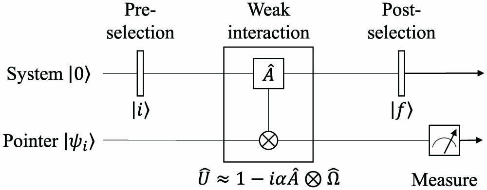
To be clear, we first consider the general weak measurement process with post-selection as depicted in Fig. 1. For simplicity, we consider a two-level system with initial state $| i ⟩$ and a pointer with initial state $| ψ_{i} ⟩$ . They couple together during the weak interaction procedure with an impulse Hamiltonian ${\hat{H}}_{I} = δ (t - t_{0}) α \hat{A} \otimes \hat{Ω}$ , where $\hat{Ω}$ is a translation operator on the pointer, and $α$ is the corresponding interaction strength. Here $\hat{A}$ is a Pauli operator on the two-level system. In weak measurement scheme, the interaction strength $α ≪ 1$ , and then the unitary evolution operator of weak interaction procedure can be approximately calculated as $\hat{U} = \exp (- i \int {\hat{H}}_{I} d t) \approx 1 - i α \hat{A} \otimes \hat{Ω}$ . (Without loss of generality, we adopt units making $ℏ = 1$ in this paper.)

Post-selected weak measurement scheme.

Figure 1.Post-selected weak measurement scheme.

To individually read out the measurement information from the pointer, we post-select the system by state $| f ⟩$ and turn the final state in whole to be $| ψ_{f} ⟩ | f ⟩$ , where $| ψ_{f} ⟩ \approx N (1 - i α A_{w} \hat{Ω}) | ψ_{i} ⟩$ is the pointer’s final state, and $N = 1 / \sqrt{1 + 2 α Im (A_{w}) {⟨ \hat{Ω} ⟩}_{i} + α^{2} {| A_{w} |}^{2} {⟨ {\hat{Ω}}^{2} ⟩}_{i}}$ is the normalized factor with ${⟨ \hat{Ω} ⟩}_{i} = ⟨ ψ_{i} | \hat{Ω} | ψ_{i} ⟩$ , ${⟨ {\hat{Ω}}^{2} ⟩}_{i} = ⟨ ψ_{i} | {\hat{Ω}}^{2} | ψ_{i} ⟩$ . $A_{w}$ is a weak value calculated by $A_{w} = ⟨ f | \hat{A} | i ⟩ / ⟨ f | i ⟩$ [23,24].

To analyze the estimating precision in our weak measurement scenario, we employ the quantum Fisher information (QFI) as a figure of merit [25,26]. The QFI of final pointer state $| ψ_{f} ⟩$ about interaction strength parameter $α$ can be calculated as $Q (α) \approx 4 {| A_{w} |}^{2} {⟨ Δ {\hat{Ω}}^{2} ⟩}_{i}$ , where ${⟨ Δ {\hat{Ω}}^{2} ⟩}_{i} = {⟨ {\hat{Ω}}^{2} ⟩}_{i} - {⟨ \hat{Ω} ⟩}_{i}^{2}$ . For $N$ classical measured samples, the variance of estimator $\hat{α}$ satisfies the QCR inequality $δ {\hat{α}}^{2} \geq 1 / N Q (α)$ , which leads to an uncertainty relation $δ {\hat{α}}^{2} {⟨ Δ {\hat{Ω}}^{2} ⟩}_{i} \geq \frac{1}{4 N {| A_{w} |}^{2}} .$ (1)

In this work, we apply the weak measurement scheme to the measurement of angular rotation. Thus, the interaction strength corresponds to the rotation angle of pointer, and the translation operator $\hat{Ω} = {\hat{L}}_{z}$ is the OAM operator. Traditionally, the laser beam with a Gaussian profile is widely used in weak measurement, and the corresponding spatial wave function is $ψ_{G} (x, y) = \frac{1}{\sqrt{2 π σ_{0}^{2}}} \exp (- \frac{x^{2} + y^{2}}{4 σ_{0}^{2}})$ , where $σ_{0}^{2}$ is the spatial variance of the Gaussian beam. Obviously, ${⟨ Δ {\hat{L}}_{z}^{2} ⟩}_{G} = 0$ because of the rotational symmetry of the Gaussian beam. Thus, it is necessary to devise an appropriate pointer for rotation measurement. In addition, as revealed from Eq. (1), increasing the variance of the OAM of the pointer is beneficial for higher precision on measuring angular rotations.

For this reason, we employ the $m n$ -order HG beam as initial pointer for the measurement of angular rotations, where $m$ and $n$ are the transverse mode numbers of the $x$ component and $y$ component, respectively. Though the $m n$ -order HG beam takes zero-mean OAM [7], its variance of OAM distribution increases quadratically with the mode numbers ${⟨ Δ {\hat{L}}_{z}^{2} ⟩}_{m n} = 2 m n + m + n,$ (2)which are going to be derived from the following. Then the quantum limit of rotation measurement with the $m n$ -order HG beam is given as $δ {\hat{α}}^{2} \geq \frac{1}{4 N {| A_{w} |}^{2} (2 m n + m + n)},$ (3)which is derived from the QCR inequality (1), and the ultimate precision is improved quadratically with mode numbers $m$ and $n$ . Besides the improvement on the quantum limit of rotation measurement, employing HG beams also provides a more convenient way to implement the optimal measurement for demodulating angular rotations in a practical system.

B. Operator Algebra of HG Beams

In detail, we can relate the HG beams to the harmonic oscillators (HOs) here. The wave function of the HG beam is [27] $u_{m n} (x, y, z) = \exp [\frac{i k (x^{2} + y^{2})}{2 q (z)} - i (m + n + 1) χ (z)] \frac{σ_{0}}{σ (z)} ψ_{m n} [\frac{σ_{0}}{σ (z)} x, \frac{σ_{0}}{σ (z)} y],$ (4)where the three $z$ -dependent parameters, spatial variance $σ^{2}$ , Gouy phase $χ$ , and radius of curvature of the wavefront $q$ , can be determined by equalities $\frac{1}{2 σ^{2} (z)} - \frac{i k}{q (z)} = \frac{k}{b + i z}, \tan χ (z) = \frac{z}{b},$ (5)where $k$ is the wavenumber and $b$ is the Rayleigh range [28]. $ψ_{m n} (x, y)$ in Eq. (4) is the 2D harmonic HG function $ψ_{m n} (x, y) = \frac{H_{m} (\frac{x}{\sqrt{2} σ_{0}}) H_{n} (\frac{y}{\sqrt{2} σ_{0}})}{\sqrt{2^{m + n + 1} π σ_{0}^{2} m! n!}} \exp (- \frac{x^{2} + y^{2}}{4 σ_{0}^{2}}),$ (6)where $H_{n}$ is the $n$ -order Hermite polynomial.

From the view of quantum mechanics, wave function $ψ_{m n} (x, y)$ is the time-independent solution for the Schrödinger equation of 2D harmonic oscillators: $i \frac{\partial ψ}{\partial t} = [σ_{0}^{2} ({\hat{p}}_{x}^{2} + {\hat{p}}_{y}^{2}) + \frac{1}{4 σ_{0}^{2}} ({\hat{x}}^{2} + {\hat{y}}^{2})] ψ .$ (7)For eigenvalue $E_{m n} = m + n + 1$ , the corresponding eigenket can be obtained as $| m, n ⟩ = \int \int d x d y ψ_{m n} (x, y) | x, y ⟩ .$ (8)

Here, we denote the $m n$ -order HG beam state as $| u_{m n} (z) ⟩ = \int \int d x d y u_{m n} (x, y) | x, y ⟩ .$ (9)Obviously, $| u_{m n} (0) ⟩ = | m, n ⟩$ . We define the creation (annihilation) operators for the HO state $| m, n ⟩$ : ${\hat{a}}_{x}^{†} | m, n ⟩ = \sqrt{m + 1} | m + 1, n ⟩, {\hat{a}}_{x} | m, n ⟩ = \sqrt{m} | m - 1, n ⟩,$ (10) ${\hat{a}}_{y}^{†} | m, n ⟩ = \sqrt{n + 1} | m, n + 1 ⟩, {\hat{a}}_{y} | m, n ⟩ = \sqrt{n} | m, n - 1 ⟩ .$ (11)

HG beam states are $z$ dependent, and their wave functions are the solutions of the paraxial wave equation $- 2 i k \frac{\partial}{\partial z} u (x, y, z) = (\frac{\partial^{2}}{\partial x^{2}} + \frac{\partial^{2}}{\partial y^{2}}) u (x, y, z),$ (12)which can be rewritten as $\frac{d}{d z} | u_{n} (z) ⟩ = - \frac{i}{2 k} ({\hat{p}}_{x}^{2} + {\hat{p}}_{y}^{2}) | u_{n} (z) ⟩ .$ (13)This equation has the formal solution $| u_{m n} (z) ⟩ = \hat{U} (z) | u_{m n} (0) ⟩$ with the propagation operator $\hat{U} (z) = \exp [- \frac{i}{2 k} ({\hat{p}}_{x}^{2} + {\hat{p}}_{y}^{2}) z] .$ (14)Thus, the $z$ -dependent mode creation (annihilation) operators can be derived by ${\hat{a}}_{x} (z) = \hat{U} (z) {\hat{a}}_{x} {\hat{U}}^{†} (z), {\hat{a}}_{x}^{†} (z) = \hat{U} (z) {\hat{a}}_{x}^{†} {\hat{U}}^{†} (z),$ (15) ${\hat{a}}_{y} (z) = \hat{U} (z) {\hat{a}}_{y} {\hat{U}}^{†} (z), {\hat{a}}_{y}^{†} (z) = \hat{U} (z) {\hat{a}}_{y}^{†} {\hat{U}}^{†} (z) .$ (16)Hence, the momentum and position operators can be obtained by these $z$ -dependent creation and annihilation operators: ${\begin{cases} {\hat{p}}_{x} = - \frac{i}{2 σ_{0}} [{\hat{a}}_{x} (z) - {\hat{a}}_{x}^{†} (z)] \\ \hat{x} = σ_{0} [{\hat{a}}_{x} (z) + {\hat{a}}_{x}^{†} (z)] + \frac{z σ_{0}}{i b} [{\hat{a}}_{x} (z) - {\hat{a}}_{x}^{†} (z)] \\ {\hat{p}}_{y} = - \frac{i}{2 σ_{0}} [{\hat{a}}_{y} (z) - {\hat{a}}_{y}^{†} (z)] \\ \hat{y} = σ_{0} [{\hat{a}}_{y} (z) + {\hat{a}}_{y}^{†} (z)] + \frac{z σ_{0}}{i b} [{\hat{a}}_{y} (z) - {\hat{a}}_{y}^{†} (z)] \end{cases} .$ (17)

Moreover, it is easy to determine that the momentum operators ${\hat{p}}_{x} = - \frac{i}{2 σ_{0}} ({\hat{a}}_{x} - {\hat{a}}_{x}^{†})$ and ${\hat{p}}_{y} = - \frac{i}{2 σ_{0}} ({\hat{a}}_{y} - {\hat{a}}_{y}^{†})$ for 2D HO states, which have the same expression as those of HG beam states. In other words, the result of inflicting displacement on the $m n$ -order HG beam state is the same as that of the $m n$ -order HO state. Then we can derive the OAM operator ${\hat{L}}_{z}$ by Eq. (17): ${\hat{L}}_{z} = \hat{x} {\hat{p}}_{y} - \hat{y} {\hat{p}}_{x} = i [{\hat{a}}_{x} (z) {\hat{a}}_{y}^{†} (z) - {\hat{a}}_{x}^{†} (z) {\hat{a}}_{y} (z)] .$ (18)Obviously, the OAM variance of the $m n$ -order HG beam ${⟨ Δ {\hat{L}}_{z}^{2} ⟩}_{m n} = 2 m n + m + n$ is $z$ independent, and the OAM operator ${\hat{L}}_{z}$ is also $z$ independent because ${\hat{L}}_{z} \equiv \hat{U} (z) {\hat{L}}_{z} {\hat{U}}^{†} (z)$ . Thus, the $m n$ -order HG beam state is equivalent to the $m n$ -order HO state in the scenario of rotation measurement.

C. Saturating Quantum Limit via Projective Measurement

Taking the initial pointer state as $| ψ_{i} ⟩ = | m, n ⟩$ , then the final pointer state can be calculated as $| ψ_{f} ⟩ \approx | m, n ⟩ + A_{w} α [\sqrt{m (n + 1)} | m - 1, n + 1 ⟩ - \sqrt{(m + 1) n} | m + 1, n - 1 ⟩],$ (19)where the rotation parameters are carried by an HG mode state $| ψ_{\hat{L}} ⟩ = \frac{1}{\sqrt{2 m n + m + n}} [\sqrt{m (n + 1)} | m - 1, n + 1 ⟩ - \sqrt{(m + 1) n} | m + 1, n - 1 ⟩],$ (20)which is a superposition state of pointer’s adjacent modes $| m - 1, n + 1 ⟩$ and $| m + 1, n - 1 ⟩$ .

In a complete metrological process, a classical measurement strategy is necessary for the final state to read out the unknown parameters [29]. In this case, the final estimating precision of angular rotation is evaluated by the classical Fisher information (CFI): $F (α) = \sum_{λ} \frac{1}{⟨ ψ_{f} | {\hat{Π}}_{λ} | ψ_{f} ⟩} {(\frac{\partial}{\partial α} ⟨ ψ_{f} | {\hat{Π}}_{λ} | ψ_{f} ⟩)}^{2},$ (21)where $\hat{Π} = {{\hat{Π}}_{λ} | \hat{Π} \geq 0, \sum_{λ} {\hat{Π}}_{λ} = \hat{I}}$ is a set of positive-operator-valued measure (POVM). Then the practical precision of angular rotation is limited by the classical Cramér–Rao (CCR) bound $δ {\hat{α}}^{2} \geq 1 / N F (α)$ . Basically, the CCR bound of a single parameter is capable of saturating the quantum limit given by QCR inequality via devising an optimal measurement strategy [29]. For the measurement of angular rotation, the tomography of OAM distributions ${\hat{Π}}_{OAM} = {| l ⟩ ⟨ l | | l \in Z}$ was usually chosen as the optimal POVM traditionally [17], where $| l ⟩$ is the eigenket of the OAM operator. However, the complete tomography theoretically requires infinite projective measurements on different eigenkets $| l ⟩$ for final pointer. In our scheme with an $m n$ -order HG pointer, a single projection for final pointer on the state $| ψ_{\hat{L}} ⟩$ is capable of demodulating the angular rotations, and the tomography of the OAM spectrum or HG mode spectrum is no longer required. Especially, no matter how large the mode number of initial HG pointer is, the optimal POVM on the final pointer is a single projective measurement ${\hat{Π}}_{HG} = {{\hat{Π}}_{\hat{L}} = | ψ_{\hat{L}} ⟩ ⟨ ψ_{\hat{L}} |, \hat{I} - {\hat{Π}}_{L}}$ . Then the CFI of the rotation parameter can be calculated as $F (α) = 4 {| A_{w} |}^{2} (2 m n + m + n)$ , which leads to the CCR bound $δ {\hat{α}}^{2} \geq 1 / 4 N {| A_{w} |}^{2} (2 m n + m + n)$ saturating the corresponding QCR bound in Eq. (3). To visualize the dependency of the theoretical precision limit on the mode numbers $m$ and $n$ , we illustrate the CCR bound of parameter $α$ with different mode numbers under projective measurement method in Fig. 2, where the measured number of photons is set as $N = 4.04 \times 10^{7}$ and the weak value is set as $A_{w} = \cot 5 ° \approx 11$ . Besides, we also plot the CCR bound at $m = n$ with the red line in Fig. 2, where the precision limit is improved fastest, and the dependency of the sensitivity on the factor of $2 m n + m + n$ is evident.

Figure 2.Lower bound of estimation variances $δ {\hat{α}}^{2}$ with different mode numbers under the projective measurement method. The measured photons number is set as $N = 4.04 \times 10^{7}$ , and the weak value is set as $A_{w} = \cot 5^{°} \approx 11$ . The $x$ axis and $y$ axis are the mode numbers of $m$ and $n$ , respectively, and the $z$ axis is the estimation variance of parameter $α$ . The red line in this figure is the CCR bound at $m = n$ , where the precision limit is improved fastest.

3. EXPERIMENTAL SCHEME

A. Experimental Materials and Setup

To experimentally verify that the enhancement on rotation measurement with an HG pointer, we setup a practical optical system to implement it as shown in Fig. 3. A light beam from a laser working at 780 nm is expanded and then converted to $m n$ -order HG mode via a spatial light modulator (SLM) and a spatial filter system [30]. Here the beam’s polarization states $| H ⟩$ and $| V ⟩$ are set as the basis of the two-level system. We employ a Dove prism to introduce a pair of inverse weak rotations $α$ for the $| H ⟩$ and $| V ⟩$ components in a polarizing Sagnac interferometer. The Pauli operator is denoted as $\hat{A} = | H ⟩ ⟨ H | - | V ⟩ ⟨ V |$ . In the post-selected weak measurement scheme, pre-selection and post-selection states are nearly orthogonal to amplify the estimated parameter [17,31 –35]. Thus, we choose $| i ⟩ = \frac{1}{\sqrt{2}} (| H ⟩ + | V ⟩)$ and $| f ⟩ = \cos (\frac{π}{4} - ε) | H ⟩ - \sin (\frac{π}{4} - ε) | V ⟩$ , where $ε ≪ 1$ . Thus, the weak value $A_{w} = \cot ε$ . Considering $N$ measurement samples (effective measured number of photons in the experiment), the minimum detectable rotation $α$ given by QCR bound is $α_{\min}^{QCR} = \frac{1}{\sqrt{2 m n + m + n}} \frac{1}{2 | \cot ε | \sqrt{N}},$ (22)which is significantly improved by the spatial mode numbers of the HG beams.

Figure 3.Diagram of the experimental setup. (a) The $m n$ -order HG beam is converted from an expanded Gaussian beam of an 780 nm laser by an SLM and a spatial filter system. The pre-selection is implemented by a Glan–Taylor polarizer (GTP) and an HWP. A polarized Sagnac interferometer is employed to implement the weak interaction procedure, where the inverse rotation signals are introduced by a Dove prism. Then a Soleil–Babinet compensator (SBC), an HWP, and a GTP are used to implement the post-selection. Finally, another SLM with a Fourier transfer lens is used to implement the projective measurement, where the successful projected photons are collected by an APD with an SMF. (b) Dove prism with PZT chips and generation method of the rotation signal. There are four PZT chips pasted on the reflection side of the prism with a $2 \times 2$ array, where the vertical distance of the PZT array is 10 mm.

The laser employed in this experiment is a distributed Bragg reflector (DBR) single-frequency laser of Thorlabs Inc. (part number: DBR780PN), which works at 780 nm with 1 MHz typical linewidth. To generate the high-order HG beams, we used an SLM of Hamamatsu Photonics (part number: X13138-02), which has $1272 \times 1024$ pixels with 12.5 μm pixel pitch. The focal length of the Fourier lens in the $4 f$ system is 5 cm. A 200 μm square pinhole is used as the spatial filter.

In this work, we set up a polarized Sagnac interferometer to introduce a pair of inverse rotation signals for horizontal and vertical polarization states. However, the extinction ratio of the reflection port of the polarizing beam splitter (PBS) cube (part number CCM1-PBS25-780/M of Thorlabs Inc.) is from 20:1 to 100:1 in practice, which deteriorates the degree of polarization of the output beam. Hence, we added a polarizer behind the reflection port of the PBS to improve the degree of polarization. A half-wave plate (HWP), whose optic axis is at 45° angle with respect to the horizontal plane, was employed to exchange the polarization states in the clockwise loop and counterclockwise loop.

In our experimental scheme, the Dove prism is driven by piezoelectric transducer (PZT) chips, and we exert an $f = 1 kHz$ cosine driving signal on the PZT to generate the tiny rotation signal. Here, we pasted four PZT chips on the reflection side of the Dove prism as illustrated in Fig. 3(b). The four PZT chips are arranged as a $2 \times 2$ array, and the vertical distance of this array is 10 mm. Here we used the NAC2013 PZT chip of the Core Tomorrow company, which shifts 22 nm with 1 V driving voltage. We exert cosine signals (with 1/2 amplitude DC bias) on the PZT chips, where a $π$ -phase difference is introduced between the top-row PZT chips and bottom-row PZT chips. Therefore, a cosine driving signal with 1 V peak-to-peak voltage corresponds to a 2.2 μrad maximum rotation of the Dove prism, which leads to a 4.4 μrad transverse rotation of the input light beam. Besides this cosine driving signal, the initial rotation bias of the Dove prism, which is denoted as $α_{0}$ and on the milliradian (mrad) scale, is non-negligible. Thus, the total rotation is $α_{tot} = α_{0} + α \cos (2 π f t)$ , and it is easy to determine that $α ≪ α_{0} ≪ 1$ .

After the post-selection, another SLM is employed to project the final pointer to carrying state $| ψ_{\hat{L}} ⟩$ with a Fourier transfer lens and a spatial filter from single-mode fiber (SMF) coupling detected photons to an avalanche photodiode (APD, part number: APD440A of Thorlabs Inc.), which has maximum conversion gain of $2.65 \times 10^{9} V/W$ and 100 kHz bandwidth. Then the detected voltage signal is analyzed by the spectrum analyzer module of Moku:Lab, which is a reconfigurable hardware platform produced by Liquid Instruments. The resolution bandwidth (RWB) of spectrum analyzer was 9.168 Hz in our experiment, which leads to the detecting time of $τ = 109.08 ms$ .

B. Experimental Results

In practice, before exerting the driving signal, we project the final pointer to state $| m, n ⟩$ to fix the measured photons number $N$ for different HG pointers. In the experiment, the detected power of the APD is fixed as $I_{0} = 94.34 pW$ at the beforehand projection step. Theoretically, the detected optical power is given as $I_{0} = γ N / τ$ , where $γ$ is the energy of a single photon at $λ = 780 nm$ and the detecting time duration $τ = 109.08 ms$ in our experiment. Thus, the effective measured photons number is fixed as $N = 4.04 \times 10^{7}$ in this experiment.

Then, exerting the driving signal on the PZT chips and projecting the final pointer to $| ψ_{\hat{L}} ⟩$ , the detected photons number is $N_{α} = {| ⟨ ψ_{\hat{L}} | {\hat{Π}}_{\hat{L}} | ψ_{\hat{L}} ⟩ |}^{2} N = (2 m n + m + n) {(\cot ε)}^{2} α_{tot}^{2} N \approx (2 m n + m + n) {(\cot ε)}^{2} α_{0}^{2} N + 2 (2 m n + m + n) {(\cot ε)}^{2} α_{0} α \cos (2 π f t) N .$ (23)Similarly, the detected power of the APD is $I_{α} \approx (2 m n + m + n) {(\cot ε)}^{2} α_{0}^{2} I_{0} + 2 (2 m n + m + n) {(\cot ε)}^{2} α_{0} α \cos (2 π f t) I_{0} .$ (24)Inputting the detected power signal of the APD into a spectrum analyzer, the tiny rotation signal at $f = 1 kHz$ is demodulated as $I_{α}^{1 kHz} = 2 (2 m n + m + n) {(\cot ε)}^{2} α_{0} α I_{0} .$ (25)From Eq. (23), we can obtain the shot noise of APD as $δ N_{α} = \sqrt{N_{α}} \approx \sqrt{2 m n + m + n} | \cot ε | α_{0} \sqrt{N}$ , and the corresponding shot-noise power is $δ I_{α} = γ δ N_{α} / τ \approx γ \sqrt{2 m n + m + n} | \cot ε | α_{0} \sqrt{N} / τ .$ (26)Thus, the detected peak signal-to-noise ratio of the spectrum analyzer is $SNR = \frac{I_{α}^{1 kHz}}{δ I_{α}} = 2 \sqrt{2 m n + m + n} | \cot ε | \sqrt{N} α .$ (27)When $SNR = 1$ , the minimum detectable rotation signal can be obtained as $α_{\min}^{(m, n)} = \frac{1}{\sqrt{2 m n + m + n}} \frac{1}{2 | \cot ε | \sqrt{N}} .$ (28)

In practice, we detected the peak level from spectrum analyzer at 1 kHz to demodulate the amplitude of rotation signal. Generally, the peak level consists of three parts: signal level, shot-noise floor, and electrical-noise floor, which is denoted as $V_{p} = V_{α} + V_{s n} + V_{e n}$ . Here, $V_{α} \propto I_{α}^{(1 kHz)}$ is the signal level, $V_{s n} \propto δ I_{α}$ is the shot-noise level, and they vary with the different HG modes. In our experiment, the electrical noise level $V_{e n} = 35.75 μV$ is a constant value in the experiment, which was detected without inputting light on the APD. The detected level of the total noise floor with a $m n$ -order HG beam is $V_{noise}^{(m, n)} = V_{s n}^{(m, n)} + V_{e n}$ . Thus, the detected signal-to-noise ratio with a $m n$ -order HG beam in our scheme is obtained as ${SNR}^{(m, n)} = \frac{V_{α}^{(m, n)}}{V_{s n}^{(m, n)}} = \frac{V_{p}^{(m, n)} - V_{noise}^{(m, n)}}{V_{noise}^{(m, n)} - V_{e n}} .$ (29)To determine the detected noise levels, we illustrate the electrical spectra of HG11 to HG66 modes at 500 Hz to 5 kHz with driving voltage 5 V in Fig. 4.

Figure 4.Detected electrical spectrum of HG11 to HG66 modes at 500 Hz to 5 kHz. The driving voltage of the PZT is 5 V, which corresponds to 22 μrad rotation signal. The first line is the spectrum of the electrical-noise floor of the APD detector, which is detected without input light on the APD.

As is shown in Fig. 4, the electrical noise is $V_{e n} = 35.75 μV$ , and the detected shot-noise level of the $m n$ -order HG beam can be calculated by $V_{s n}^{(m, n)} = V_{noise}^{(m, n)} - V_{e n}$ . We list the results in Table 1.Table 1.

Experimental Results of Detected Noise Levels

HG mode	HG11	HG22	HG33	HG44	HG55	HG66
Noise level^a	41.43 μV	44.43 μV	49.39 μV	54.08 μV	57.27 μV	61.70 μV
Shot-noise level	5.68 μV	8.68 μV	13.64 μV	18.33 μV	21.52 μV	25.95 μV

Total detected noise levels in the APD.

Figure 5.Experimental results. (a) Detected peak signal level of the HG11, HG33, and HG55 modes at 1 kHz. (b) Detected signal-to-noise ratio of the HG11, HG33, and HG55 modes. The driving voltage of the PZT increases from 0 to 2 V, which corresponds to 0–8.8 μrad rotation signal.

4. DISCUSSION

A. Technical Advantages of a Weak Value

In the theoretical frame, the post-selection is employed for individually reading out the measurement parameters from the pointer, and the precision enhancement comes from the mode entanglement of the HG pointer, but not the weak values. Thus, our main conclusion still holds in the post-selection-free scheme. In the experimental scheme, we still employed the weak value amplification technology, though the weak value $A_{w} = \cot ε$ takes no enhancement for the theoretical minimum detectable rotation in Eq. (28) because the detected number of photons $N = {| ⟨ f | i ⟩ |}^{2} N_{0} = \sin^{2} ε N_{0}$ is attenuated by the post-selection, where $N_{0}$ is the number of photons before post-selection. However, the weak value amplification technology has been proved efficient for suppressing technical noises, such as reflection of optical elements [35] and detector saturation [36,37]. The detector saturation is non-negligible in our experiment since the saturation power of our APD detector is only 1.54 nW. Considering the projection demodulation of SLM, only 10% of photons can be modulated on the first-order diffraction, so the maximum efficient received power of our detector is about 154 pW, which is easily saturated without post-selection. For example, the efficient detected light power in our experiment is $I_{0} = 94.34 pW$ , and the post-selection angle $ε = 5 °$ . Therefore, for the post-selection-free scheme, an $I_{0} / \sin^{2} ε = 12.42 nW$ detected light power is needed to achieve the same precision of the post-selected scheme, which is far larger than the saturation power of the APD detector.

B. Rotation-Coupling Weak Measurement for Hamiltonian Estimation

Though we only investigate the enhanced measurement on angular rotation, the precision enhancement of employing HG pointers can be applied in various missions in quantum physics. The most obvious application of our scheme in quantum physics is the estimation of Hamiltonian [38,39]. In this case, we do not only concentrate on the interaction strength parameter $α$ but we are also interested in the information of operator $\hat{A}$ . For a two-level system, the unknown operator can be represented as $\hat{A} = \vec{n} \cdot \vec{σ}$ , where $\vec{n} = (\sin θ \cos ϕ, \sin θ \sin ϕ, \cos θ)$ is the direction vector of the measurement operator, and $\vec{σ} = ({\hat{σ}}_{x}, {\hat{σ}}_{y}, {\hat{σ}}_{z})$ , where ${\hat{σ}}_{x}$ , ${\hat{σ}}_{y}$ , and ${\hat{σ}}_{z}$ are Pauli matrices. Thus, there are two unknown parameters $θ$ and $ϕ$ to be estimated for identifying the operator $\hat{A}$ . As we calculated in the theoretical model, the final pointer’s state in our post-selected scheme is $| ψ_{f} ⟩ \approx N (1 - i α A_{w} \hat{Ω}) | ψ_{i} ⟩$ . Then the QFI of parameter $g \in (θ, ϕ)$ can be calculated as $Q (g) \approx 4 α^{2} {| \partial_{g} A_{w} |}^{2} {⟨ Δ {\hat{Ω}}^{2} ⟩}_{i}$ . Combined with the QCR inequality $δ {\hat{g}}^{2} \geq 1 / N Q (g)$ , the estimation precision of parameter $g \in (θ, ϕ)$ satisfies the uncertainty relation $δ {\hat{g}}^{2} {⟨ Δ {\hat{Ω}}^{2} ⟩}_{i} \geq \frac{1}{4 N α^{2} {| \partial_{g} A_{w} |}^{2}},$ (30)where the quantum limits of Hamiltonian parameters are still governed by the variance of the translation operator on the initial pointer. This means that our scheme has potential to be applied in this scenario for improving the performance of Hamiltonian estimation. For example, the initial pointers with Gaussian profile are employed traditionally, and the two-level system couples with the pointer via a displacement interaction $\hat{Ω} = {\hat{p}}_{x}$ . Then the variances ${⟨ Δ {\hat{Ω}}^{2} ⟩}_{i} = {⟨ Δ {\hat{p}}_{x}^{2} ⟩}_{G} = 1 / 4 σ_{0}$ , and the corresponding quantum limit on estimating Hamiltonian parameters $g \in (θ, ϕ)$ is given by $δ {\hat{g}}^{2} \geq \frac{σ_{0}^{2}}{N α^{2} {| \partial_{g} A_{w} |}^{2}} .$ (31)If we replace the Gaussian pointer by an $m n$ -order HG pointer, the quantum limit will be improved to $δ {\hat{g}}^{2} \geq \frac{σ_{0}^{2}}{(2 m + 1) N α^{2} {| \partial_{g} A_{w} |}^{2}}$ (32)because the variance ${⟨ Δ {\hat{p}}_{x}^{2} ⟩}_{m n} = (2 m + 1) / 4 σ_{0}$ increases linearly with the HG mode $m$ in the corresponding displacement direction. Further, replacing the displacement interaction by rotational interaction, that is, $\hat{Ω} = {\hat{L}}_{z}$ , there will be a significant improvement in the precision limit on estimating Hamiltonian parameters: $δ {\hat{g}}^{2} \geq \frac{1}{4 (2 m n + m + n) N α^{2} {| \partial_{g} A_{w} |}^{2}},$ (33)which is quadratically improved by the HG mode numbers $m$ and $n$ . Moreover, the enhancement factor $2 m n + m + n$ is analog to the Heisenberg scaling limit in quantum interference [40] because the mode number $m$ in the $x$ direction and mode number $n$ in the $y$ direction are independent for an HG beam state or a 2D HO state. Thus, mode state $| m, n ⟩$ can be regarded as an eigenket in the product Hilbert space $H_{x} \otimes H_{y}$ , where $H_{x}$ and $H_{y}$ are the Hilbert spaces for the mode state in the $x$ direction and the mode state in the $y$ direction. Therefore, the OAM operator ${\hat{L}}_{z} = i ({\hat{a}}_{x} {\hat{a}}_{y}^{†} - {\hat{a}}_{x}^{†} {\hat{a}}_{y})$ in this product Hilbert space $H_{x} \otimes H_{y}$ , which leads to the unknown parameters $(α, θ, ϕ)$ taken by the state $| ψ_{\hat{L}} ⟩$ . Moreover, it is obvious to note that the state $| ψ_{\hat{L}} ⟩$ in Eq. (20) is a mode-entangled state in the product Hilbert space $H_{x} \otimes H_{y}$ .

C. Rotation-Coupling Weak Measurement for Monitoring the Quantum Bit

Besides Hamiltonian estimation, our precision-enhanced method also has the potential for monitoring the quantum bit, which is a vital mission in quantum metrology [41]. Generally, the state of an arbitrary quantum bit (qubit) can be represented as $| qubit ⟩ = \cos \frac{θ}{2} | 0 ⟩ + e^{i ϕ} \sin \frac{θ}{2} | 1 ⟩,$ (34)where $θ$ and $ϕ$ are the azimuthal angles on the Bloch sphere, and $| 0 ⟩$ and $| 1 ⟩$ are the eigenkets of Pauli operator ${\hat{σ}}_{z}$ . To avoid apparent disturbance on the qubit, a series of continuous weak measurements is adopted to monitor it [42].

As is illustrated in Fig. 6, an ancillary device (pointer) is employed to monitor the quantum system via a weak interaction procedure, which is described by the von Neumann measurement theory [23] via an impulse Hamiltonian (here we take the monitoring of qubits on the basis of ${\hat{σ}}_{z}$ , for example): ${\hat{H}}_{I} = δ (t - t_{0}) α {\hat{σ}}_{z} \otimes \hat{Ω},$ (35)which leads to a composite unitary evolution $\hat{U} = \exp (- i \int {\hat{H}}_{I} d t) \approx 1 - i α {\hat{σ}}_{z} \otimes \hat{Ω}$ of the quantum system and pointer. After the weak interaction, the measurement information of the Pauli operator ${\hat{σ}}_{z}$ on the qubit is transferred to the pointer shift of the ancillas via a translation operator $\hat{Ω}$ , and the final state of the whole system is $| Ψ_{f} ⟩ = \cos \frac{θ}{2} | 0 ⟩ | ψ_{+} ⟩ + e^{i ϕ} \sin \frac{θ}{2} | 1 ⟩ | ψ_{-} ⟩,$ (36)where $| ψ_{+} ⟩ = \exp (- i α \hat{Ω}) | ψ_{i} ⟩$ and $| ψ_{-} ⟩ = \exp (i α \hat{Ω}) | ψ_{i} ⟩$ . Unlike our post-selected weak measurement scheme, post-selection of the qubit is forbidden. Thus, we should measure the information about parameter $θ$ from the final pointer state, which is a mixed state: ${\hat{ρ}}_{f} = \cos^{2} \frac{θ}{2} | ψ_{+} ⟩ ⟨ ψ_{+} | + \sin^{2} \frac{θ}{2} | ψ_{-} ⟩ ⟨ ψ_{-} |,$ (37)and then the corresponding QFI of parameter $θ$ can be calculated as $Q (θ) = 1 - {(Re ⟨ ψ_{+} | ψ_{-} ⟩)}^{2} \approx 4 α^{2} {⟨ {\hat{Ω}}^{2} ⟩}_{i}$ , which leads to the quantum limit on measuring parameter $θ$ being governed by the uncertainty relation (see Appendix B for derivation) $δ {\hat{θ}}^{2} {⟨ {\hat{Ω}}^{2} ⟩}_{i} \geq \frac{1}{4 α^{2} N},$ (38)which means that the monitoring sensitivity is still dependent on the devising of the pointer and coupling method. Applying our $m n$ -order HG pointer and rotation-coupling method to this scheme, the quantum limit on monitoring the azimuthal angle $θ$ of the qubit is then derived as $δ {\hat{θ}}^{2} \geq \frac{1}{4 α^{2} (2 m n + m + n) N},$ (39)where the precision enhancement still holds.

Figure 6.Schematic of monitoring quantum bits.

Moreover, we express the HG beams via harmonic oscillator model, which has been widely used in quantum computation and metrology topics, such as superconducting qubits [43,44] and optomechanics [45 –47]. Thus, our theoretical model can be applied in such scenarios naturally and can provide a significant method in quantum metrology.

5. CONCLUSION

In summary, we have implemented a practical scheme for measuring the tiny rotation by employing an $m n$ -order HG pointer in a post-selected weak measurement scheme, where the precision limit is theoretically improved by a factor of $2 m n + m + n$ . Experimentally, we demodulate the angular rotation parameter via a single projective measurement, and precision up to 0.89 μrad is achieved with $5 \times 5$ -order HG beams. Moreover, we have found that the precision enhancement of the rotation-coupling method with an HG pointer still holds in a wide range of applications in quantum physics, such as Hamiltonian estimation and monitoring qubits. Thus, our results constitute valuable resources not only for measurement and control of light’s angular rotation in optical metrology but also for sensitive estimating and control of evolution procedure in quantum physics.

Acknowledgment

Acknowledgment. We thank Lijian Zhang and Kui Liu for the helpful discussions.

APPENDIX A: DERIVATION OF QUANTUM LIMITS IN A POST-SELECTED WEAK MEASUREMENT SCHEME

α

| Ψ_{i} ⟩ = | ψ_{i} ⟩ | i ⟩

| ψ (g) ⟩

\vec{n} = (\sin θ \cos ϕ, \sin θ \sin ϕ, \cos θ)

x

Figure 7.QCR bounds of the measurement parameters. (a) QCR bounds of parameter $α$ . (b) QCR bounds of parameter $θ$ . (c) QCR bounds of parameter $ϕ$ . The $y$ axis is the variance of estimator $\hat{g}$ , and the $x$ axis is the mode numbers. Mode numbers $m$ and $n$ simultaneously increase from 0 to 25. The red dotted line is the QCR bound of the Gaussian pointer with displacement coupling. The blue line is the QCR bound of the HO pointer with displacement coupling. The orange line is the QCR bound of the HO pointer with rotation coupling. Here the pre-selection state and post-selection state are chosen as $| i ⟩ = | f ⟩ = \frac{1}{\sqrt{2}} (| 0 ⟩ + e^{i \frac{π}{4}} | 1 ⟩)$ , and values of all the parameters are $α = 0.001$ , $θ = π / 4$ , and $ϕ = 0$ . In addition, the value of $σ_{0}$ is normalized to $1 / \sqrt{2}$ .

Figure 8.QCR bound of $α$ about post-selection angle $ε$ . This is the QCR bound of $α$ with a 2D HO pointer and rotation coupling. The $x$ axis is the mode numbers $m$ and $n$ , which simultaneously increase from 1 to 25. The pre-selection state is $| i ⟩ = \frac{1}{\sqrt{2}} (| 0 ⟩ + e^{i \frac{π}{4}} | 1 ⟩)$ , and the post-selection state is $| f ⟩ = \frac{1}{\sqrt{2}} (| 0 ⟩ - e^{i (\frac{π}{4} + ε)} | 1 ⟩)$ , where the angle $ε$ varies from 0.1 to 0.01. In addition, we plot three QCR bounds at different values of $ε$ . The green line is $ε = 0.1$ , the red line is $ε = 0.05$ , and the yellow line is $ε = 0.01$ .

APPENDIX B: DERIVATION OF QFI FOR MONITORING QUBITS WITH A WEAK MEASUREMENT SCHEME

\hat{U} \approx 1 - i α {\hat{σ}}_{z} \otimes \hat{Ω}

S = {| e_{1} ⟩, | e_{2} ⟩, \dots, | e_{n} ⟩}

Q (θ) = Tr ({\hat{ρ}}_{f} {\hat{L}}_{θ}^{2}) = Tr ({\hat{L}}_{θ} \partial_{θ} {\hat{ρ}}_{f}) = \sum_{| e_{x} ⟩ \in S} ⟨ e_{x} | {\hat{L}}_{θ} \partial_{θ} {\hat{ρ}}_{f} | e_{x} ⟩ = - \frac{\sqrt{1 - δ^{2}}}{2} \sin θ (⟨ e_{2} | {\hat{L}}_{θ} | e_{1} ⟩ + ⟨ e_{1} | {\hat{L}}_{θ} | e_{2} ⟩) .

APPENDIX C: GENERATION METHOD OF HG BEAMS AND EXPERIMENTAL RESULTS

4 f

A_{in} (x, y) \exp [i ϕ_{in} (x, y)]

f

Experimental Results of Generated HG Beams

HG Mode	HG00	HG11	HG22	HG33	HG44	HG55	HG66
Phase map
Simulation
Experiment
Purity	97.87%	94.91%	93.76%	92.54%	90.17%	88.24%	86.75%

APPENDIX D: IMPLEMENTATION OF PROJECTIVE MEASUREMENT

g (x, y)

| g ⟩

References

[1] J. K. Stockton, K. Takase, M. A. Kasevich. Absolute geodetic rotation measurement using atom interferometry. Phys. Rev. Lett., 107, 133001(2011).

[2] M. Padgett, R. Bowman. Tweezers with a twist. Nat. Photonics, 5, 343-348(2011).

[3] J. Courtial, D. A. Robertson, K. Dholakia, L. Allen, M. J. Padgett. Rotational frequency shift of a light beam. Phys. Rev. Lett., 81, 4828-4830(1998).

[4] M. P. J. Lavery, F. C. Speirits, S. M. Barnett, M. J. Padgett. Detection of a spinning object using light’s orbital angular momentum. Science, 341, 537-540(2013).

[5] Z. Zhang, L. Cen, J. Zhang, J. Hu, F. Wang, Y. Zhao. Rotation velocity detection with orbital angular momentum light spot completely deviated out of the rotation center. Opt. Express, 28, 6859-6867(2020).

[6] S. Shi, D.-S. Ding, Z.-Y. Zhou, Y. Li, W. Zhang, B.-S. Shi. Magnetic-field-induced rotation of light with orbital angular momentum. Appl. Phys. Lett., 106, 261110(2015).

[7] F. Pampaloni, J. Enderlein. Gaussian, Hermite-Gaussian, and Laguerre-Gaussian beams: a primer(2004).

[8] L. Allen, M. W. Beijersbergen, R. J. C. Spreeuw, J. P. Woerdman. Orbital angular momentum of light and the transformation of Laguerre-Gaussian laser modes. Phys. Rev. A, 45, 8185-8189(1992).

[9] R. Fickler, R. Lapkiewicz, W. N. Plick, M. Krenn, C. Schaeff, S. Ramelow, A. Zeilinger. Quantum entanglement of high angular momenta. Science, 338, 640-643(2012).

[10] A. K. Jha, G. S. Agarwal, R. W. Boyd. Supersensitive measurement of angular displacements using entangled photons. Phys. Rev. A, 83, 053829(2011).

[11] F. Bouchard, P. de la Hoz, G. Björk, R. W. Boyd, M. Grassl, Z. Hradil, E. Karimi, A. B. Klimov, G. Leuchs, J. Řeháček, L. L. Sánchez-Soto. Quantum metrology at the limit with extremal majorana constellations. Optica, 4, 1429-1432(2017).

[12] V. D’Ambrosio, N. Spagnolo, L. Del Re, S. Slussarenko, Y. Li, L. C. Kwek, L. Marrucci, S. P. Walborn, L. Aolita, F. Sciarrino. Photonic polarization gears for ultra-sensitive angular measurements. Nat. Commun., 4, 2432(2013).

[13] I. Afek, O. Ambar, Y. Silberberg. High-noon states by mixing quantum and classical light. Science, 328, 879-881(2010).

[14] G. Y. Xiang, B. L. Higgins, D. W. Berry, H. M. Wiseman, G. J. Pryde. Entanglement-enhanced measurement of a completely unknown optical phase. Nat. Photonics, 5, 43-47(2011).

[15] B. L. Higgins, D. W. Berry, S. D. Bartlett, H. M. Wiseman, G. J. Pryde. Entanglement-free Heisenberg-limited phase estimation. Nature, 450, 393-396(2007).

[16] R. Barboza, A. Babazadeh, L. Marrucci, F. Cardano, C. de Lisio, V. D’Ambrosio. Ultra-sensitive measurement of transverse displacements with linear photonic gears. Nat. Commun., 13, 1080(2022).

[17] O. S. Magaña Loaiza, M. Mirhosseini, B. Rodenburg, R. W. Boyd. Amplification of angular rotations using weak measurements. Phys. Rev. Lett., 112, 200401(2014).

[18] V. Delaubert, N. Treps, M. Lassen, C. C. Harb, C. Fabre, P. K. Lam, H.-A. Bachor. tem₁₀ homodyne detection as an optimal small-displacement and tilt-measurement scheme. Phys. Rev. A, 74, 053823(2006).

[19] H. Sun, K. Liu, Z. Liu, P. Guo, J. Zhang, J. Gao. Small-displacement measurements using high-order Hermite-Gauss modes. Appl. Phys. Lett., 104, 121908(2014).

[20] A. Holevo. Unbiased Measurements, 219-264(2011).

[21] C. Rosales-Guzmán, N. Hermosa, A. Belmonte, J. P. Torres. Experimental detection of transverse particle movement with structured light. Sci. Rep., 3, 2815(2013).

[22] N. Uribe-Patarroyo, A. Fraine, D. S. Simon, O. Minaeva, A. V. Sergienko. Object identification using correlated orbital angular momentum states. Phys. Rev. Lett., 110, 043601(2013).

[23] Y. Aharonov, D. Z. Albert, L. Vaidman. How the result of a measurement of a component of the spin of a spin-1/2 particle can turn out to be 100. Phys. Rev. Lett., 60, 1351-1354(1988).

[24] R. Jozsa. Complex weak values in quantum measurement. Phys. Rev. A, 76, 044103(2007).

[25] K. Matsumoto. A new approach to the Cramér-Rao-type bound of the pure-state model. J. Phys. A, 35, 3111-3123(2002).

[26] R. Demkowicz-Dobrzański, M. Jarzyna, J. Kołodyński. Chapter 4 - Quantum limits in optical interferometry. Prog. Opt., 60, 345-435(2015).

[27] I. Kimel, L. R. Elias. Relations between Hermite and Laguerre Gaussian modes. IEEE J. Quantum Electron., 29, 2562-2567(1993).

[28] G. Nienhuis. Analogies between optical and quantum mechanical angular momentum. Philos. Trans. R. Soc. A, 375, 20150443(2017).

[29] J. Liu, H. Yuan, X.-M. Lu, X. Wang. Quantum fisher information matrix and multiparameter estimation. J. Phys. A: Math. Theor., 53, 023001(2019).

[30] T. W. Clark, R. F. Offer, S. Franke-Arnold, A. S. Arnold, N. Radwell. Comparison of beam generation techniques using a phase only spatial light modulator. Opt. Express, 24, 6249-6264(2016).

[31] O. Hosten, P. Kwiat. Observation of the spin Hall effect of light via weak measurements. Science, 319, 787-790(2008).

[32] P. B. Dixon, D. J. Starling, A. N. Jordan, J. C. Howell. Ultrasensitive beam deflection measurement via interferometric weak value amplification. Phys. Rev. Lett., 102, 173601(2009).

[33] M. Hallaji, A. Feizpour, G. Dmochowski, J. Sinclair, A. Steinberg. Weak-value amplification of the nonlinear effect of a single photon. Nat. Phys., 13, 540-544(2017).

[34] H. Li, J.-Z. Huang, Y. Yu, Y. Li, C. Fang, G. Zeng. High-precision temperature measurement based on weak measurement using nematic liquid crystals. Appl. Phys. Lett., 112, 231901(2018).

[35] C. Fang, J.-Z. Huang, G. Zeng. Robust interferometry against imperfections based on weak value amplification. Phys. Rev. A, 97, 063818(2018).

[36] L. Xu, Z. Liu, L. Zhang. Weak-measurement-enhanced metrology in the presence of ccd noise and saturation. Frontiers in Optics/Laser Science, JW4A.126(2018).

[37] L. Xu, Z. Liu, A. Datta, G. C. Knee, J. S. Lundeen, Y.-Q. Lu, L. Zhang. Approaching quantum-limited metrology with imperfect detectors by using weak-value amplification. Phys. Rev. Lett., 125, 080501(2020).

[38] A. Sone, P. Cappellaro. Hamiltonian identifiability assisted by a single-probe measurement. Phys. Rev. A, 95, 022335(2017).

[39] C. Fang, B. Xia, J. Huang, T. Xiao, Y. Yu, H. Li, G. Zeng. Hamiltonian estimation based on adaptive weak value amplification. J. Phys. B, 54, 075501(2021).

[40] M. Genovese. Experimental quantum enhanced optical interferometry. AVS Quantum Sci., 3, 044702(2021).

[41] Z. K. Minev, S. O. Mundhada, S. Shankar, P. Reinhold, R. Gutiérrez-Jáuregui, R. J. Schoelkopf, M. Mirrahimi, H. J. Carmichael, M. H. Devoret. To catch and reverse a quantum jump mid-flight. Nature, 570, 200-204(2019).

[42] M. Hays, V. Fatemi, K. Serniak, D. Bouman, S. Diamond, G. de Lange, P. Krogstrup, J. Nygård, A. Geresdi, M. H. Devoret. Continuous monitoring of a trapped superconducting spin. Nat. Phys., 16, 1103-1107(2020).

[43] M. D. LaHaye, J. Suh, P. M. Echternach, K. C. Schwab, M. L. Roukes. Nanomechanical measurements of a superconducting qubit. Nature, 459, 960-964(2009).

[44] M. Kjaergaard, M. E. Schwartz, J. Braumüller, P. Krantz, J. I.-J. Wang, S. Gustavsson, W. D. Oliver. Superconducting qubits: current state of play. Annu. Rev. Condens. Matter Phys., 11, 369-395(2020).

[45] A. D. O’Connell, M. Hofheinz, M. Ansmann, R. C. Bialczak, M. Lenander, E. Lucero, M. Neeley, D. Sank, H. Wang, M. Weides, J. Wenner, J. M. Martinis, A. N. Cleland. Quantum ground state and single-phonon control of a mechanical resonator. Nature, 464, 697-703(2010).

[46] B. Pepper, R. Ghobadi, E. Jeffrey, C. Simon, D. Bouwmeester. Optomechanical superpositions via nested interferometry. Phys. Rev. Lett., 109, 023601(2012).

[47] K. C. Balram, M. I. Davanço, J. D. Song, K. Srinivasan. Coherent coupling between radiofrequency, optical and acoustic waves in piezo-optomechanical circuits. Nat. Photonics, 10, 346-352(2016).

[48] W. Kong, A. Sugita, T. Taira. Generation of Hermite–Gaussian modes and vortex arrays based on two-dimensional gain distribution controlled microchip laser. Opt. Lett., 37, 2661-2663(2012).

[49] S.-C. Chu, Y.-T. Chen, K.-F. Tsai, K. Otsuka. Generation of high-order Hermite-Gaussian modes in end-pumped solid-state lasers for square vortex array laser beam generation. Opt. Express, 20, 7128-7141(2012).

[50] B. Xia, J. Huang, C. Fang, H. Li, G. Zeng. High-precision multiparameter weak measurement with Hermite-Gaussian pointer. Phys. Rev. Appl., 13, 034023(2020).