
C. Y. Qin, H. Zhang, S. Li, S. H. Zhai, A. X. Li, J. Y. Qian, J. Y. Gui, F. X. Wu, Z. X. Zhang, Y. Xu, X. Y. Liang, Y. X. Leng, B. F. Shen, L. L. Ji, R. X. Li. Mapping non-laminar proton acceleration in laser-driven target normal sheath field[J]. High Power Laser Science and Engineering, 2022, 10(1): 010000e2
- High Power Laser Science and Engineering
- Vol. 10, Issue 1, 010000e2 (2022)
Abstract
Keywords
1 Introduction
Laser-driven target normal sheath acceleration (TNSA) is a very robust mechanism for generating proton sources at tens of megaelectronvolts energy with ultralow transverse emittance (e.g., better than 0.004 mm∙mrad in Ref. [1]). Such highly directional proton beams are advantageous in various applications such as probing high-energy-density states[2], treating cancer therapy[3], and fast ignition fusion[4]. As the TNSA facilitates compact, stable, and affordable proton sources[5], full understanding of the beam properties becomes crucial. Usually, the proton beams accelerated from TNSA expand into vacuum in a self-similar manner[6] and are of high degree of laminarity[1]. In other words, protons at a same position have identical transverse velocities and their orbits do not cross each other[7]. Laminar beams have outstanding transport properties that can support micro-sized spot sizes, a highly favored feature in sequential applications.
However, proton beams can be significantly modulated via, for instance, Weibel-like instability (WI) during laser–plasma interaction[8–10]. Experimental and simulation studies show that pre-plasma can be created by laser pre-pulse on the target rear surface[8,10,11] or the front[12]. WI or electron filamentation instability spontaneously arises from laser-driven fast electrons streaming in background plasma[13–16]. The electron beam profile is further mapped onto the proton beam during acceleration[10,17]. Such filamentations could be diagnosed either from the spatially modulated proton beams accelerated by the sheath field[17,18] or the transition radiation induced by fast electrons[19]. It is usually associated with strong magnetic field (B ~ 100 MG) as probed via magneto-optic polarograms[20].
A filamented profile is regarded as a key sign of disrupted laminarity[8,10]. These signals can be regularly obtained using radiochromic film (RCF) detectors. To identify whether these modulated protons are from near-axis or off-axis and further reveal the size of the perturbed area, we propose to implement the knife-edge technique (KET)[21] into the RCF detector in laser–proton acceleration. For laminar sources, the KET would give a virtual source size in the sense of a beam waist[22]. However, it perfectly serves our purpose because we focus on non-laminar proton feature existing in acceleration.
Sign up for High Power Laser Science and Engineering TOC. Get the latest issue of High Power Laser Science and Engineering delivered right to you!Sign up now
2 Experimental results
Using the KET-RCF method, we experimentally study the proton distribution from laser irradiating micro-sized planar aluminum targets. We observe a ring-like profile and filamentation simultaneously. The KET diagnosis reveals that the ring structure stems from low-energy protons located far off-axis, whereas the filamentation belongs to the high-energy group disturbed by WI in the near-axis area. Typical source sizes of the non-laminar protons are found to be 30–110 μm for energy of more than 5 MeV. We believe through particle-in-cell (PIC) simulations that the magnetic field evolving at two distinctive time scales is responsible for the observed features.
2.1 Experimental setup
The experiments were carried out in the Shanghai Superintense Ultrafast Laser Facility (SULF). Therein, the 1-PW laser system[23] delivers a 28-J and 35-fs (full width at half maximum, FWHM) pulse of wavelength λ = 800 nm. The pulse is focused to a beam size of 12 μm (FWHM, contains ~7.2 J energy), yielding a peak intensity of 1.8 × 10²⁰ W/cm2 on target. The laser amplified spontaneous emission (ASE) pedestal is at 10–11–10–10 level and there exists a 10–6 pre-pulse at 3 ns prior to the main pulse. This strong nanosecond pre-pulse tends to trigger a strong shock which will lead to pre-plasma at both sides of the target[24]. The experimental setup is shown in Figure 1, where the laser pulse is focused onto a 10-μm-thick aluminum target by an F/3 off-axis parabola (OAP). It is
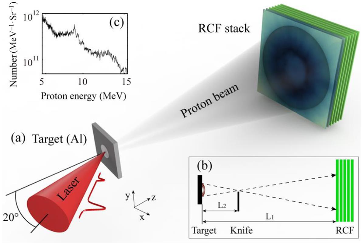
Figure 1.Sketch of the experimental setup (a) without the knife edge and (b) with the knife edge. (c) The typical proton energy spectrum of 10-μm aluminum detected by a Thomson parabolic spectrometer in a separate run. The laser pulse with 1.8 × 10²⁰ W/cm2, 35 fs, 12 μm (beam size) and 10–6@3 ns irradiates a 10-μm-thick aluminum foil at 20° incident angle.
2.2 Ring and filamentation profiles
We first remove the knife edge and let the protons fly freely towards the RCF stack. The signals at different proton energies are collected in Figure 2 (see full RCF signals in the
![]()
Figure 2.(a1)–(a4) The proton beam profiles of different energy on RCF without knife edge and (b1)–(b4) proton beam profiles of different energy on RCF with a knife edge. (c) The dose distribution along the dashed lines in (a1)–(a4). (d) The OD distribution in the white dashed rectangle in (b2). The red/blue parts denote the area irradiated/non-irradiated by protons and the transition between (yellow–green) is the penumbra region.
For more energetic protons (
2.3 Non-laminar proton beam
We further diagnose the non-laminar proton beam employing the KET to retrieve the proton source sizes at different energies. The experimental setup is shown in Figure 1(b), where we move the knife edge up to the position that is horizontal to the target center. The RCF stack used in these shots consists of two HD-V2s and eight EBT3s. Proton signals are shown in Figures 2(b1)–2(b4) where the rectangles denote the knife shadows. The proton dose distribution can be divided into three parts. The area completely irradiated by the proton source forms the dark region, whereas the non-irradiated area corresponds to the bright region. Protons pass through the knife edge following the dashed lines in Figure 1(b) producing a penumbra area in the RCF. It is a narrow strip sandwiched between the bright and dark. We take an approximately 4 mm × 2 mm knife edge area from Figure 2(b2) and show the optical density (OD) distribution in Figure 2(d). The pictures used for data processing are grayscale images scanned with a resolution of 4800 dpi. We see a clear transition area in the color map. Here the electron and X-ray irradiation background have been subtracted. The dose in the bright area is not exactly zero because the blade is not thick enough to block all protons.
Now that the width of the penumbra is known, the source size can be inferred through geometric proportional relationship. We randomly select five x-positions in Figure 2(d) and average the OD to remove noise. The edge spread function (ESF) of the OD value is plotted in Figure 3(a). The width of the penumbra is defined as d = 2(y1– y2), where y1 is the relative position corresponding to the OD value of
![]()
Figure 3.(a) The ESF function for the OD value along the direction of the vertical knife edge. The red dashed line shows the fitting curve of the averaged experiment results (black solid line) with
By implementing the KET, each RCF sheet not only records the beam profile but also the source size at a particular proton energy level. The data of the three shots with the same KET location are presented in Figure 3(b) after being averaged. Here, EBT3 sheets were mainly analyzed to avoid the influence from different RCF sensibilities. Measurements at the high-energy end give 30–50 μm source size for proton energy greater than 10 MeV. The size diagnosed here (>10 MeV) is about 3–7 times the laser spot size in FWHM. Furthermore, to confirm the KET results, we used the mesh method to calibrate the source sizes[30]. The mesh is placed parallel to the target rear surface at a distance of approximately 150 μm, and Figure 3(b) shows the sizes are about 43 and 25 μm for the energy of 11.1 and 12.7 MeV, respectively (see the details in the
3 Simulation and discussion
One possible mechanism responsible for the ring-like structure is the quasi-static annular magnetic field generated when laser ablates the target surface. Magnetic field up to 103 T can be established through laser-driven electric current and protons could be diverged or focused when passing through[33]. On the other hand, the filamentation structure is believed to be caused by WI accompanied with target-rear pre-plasma[8,10,11]. In this case, the scale length should be larger than the critical value Lp,c ≈ 0.13λ(a0)1/2~ 0.3 μm[10].
However, it is not clear why both features co-exist, with low energy protons distributed in a ring and high energy ones filamented simultaneously. Even more interesting is that the latter seems originating from the near-axis center of the interaction area thanks to the KET measurement. PIC simulations are therefore performed to reveal the underlying mechanism. We run the simulations in two dimensions using the EPOCH code[34]. The simulation box is 100 μm × 100 μm in x × y directions (x = 0–100 μm, y = –45–55 μm) with 8000 × 6250 cells. The laser pulse parameters are set to match the laboratory laser condition, which is of 0.8-μm wavelength, 35-fs duration, and 12-μm spot size. It is
When the main pulse arrives at the pre-plasma in the front, it efficiently drives energetic electrons. The latter pass through the target and stream in the pre-plasma at the rear surface. Return current grows[11] and drives WI, leading to magnetic field filamentation[20,36–39], as seen in the near-axis area in Figure 4(a) at 120 fs. The transverse motion direction of the accelerated protons is disturbed when they pass through such a magnetic field. In every filament cycle Bz changes its sign, and therefore protons are deflected in the opposite transverse direction. From Figure 4(e) we see that the transverse momenta are staggered such that their orbits intersect later in this vicinity and form a strong non-laminar flow. At 400 fs, the WI-induced magnetic field vanishes as shown in Figure 4(c). The proton density already forms significant filaments, with featured spatial period about 1.3 μm (Figure 4(f)). From Figures 4(b) and 4(d) we can see that background electron shows filamentation after a longer time of evolution. As the plasma expands further, the magnetic field from filamentation decays whereas the large-scale magnetic field from the thermoelectric effect is sustained for a much longer time. Theoretical analysis suggests that the Weibel separated filament thickness should be of the order of
![]()
Figure 4.Results from PIC simulations. The magnetic field distribution along the
![]()
Figure 5.(a) Evolution of the
In our simulations, magnetic filamentation occurs at approximately 100 fs, boosting the field strength to 104 T in less than 100 fs. The field then rapidly drops to approximately 103 T, which can be seen in Figure 5(a). On the other hand, a long-term azimuthal magnetic field of hundreds of tesla persists in the far-axis area; see Figures 4(a), 4(c), and 5(a). The strong quasi-static B-fields are mainly generated by laser-driven electric currents, which last for picoseconds before getting damped[33,41]. Figure 5(a) shows the net current density Jx along the –x direction declining in about 1 ps. The corresponding magnetic field is estimated using Bcal
This magnetic field could extend to 3–5 μm length scale and provides a bending force that deflects the far-axis protons (usually of low energy) sideways. Essentially, they form a ring-like structure in space. When the 1 MeV protons pass through a uniform magnetic field (consider Bz
4 Conclusion
In conclusion, through direct mapping of protons with the KET-RCF method and PIC simulations, we have found that energetic electrons streaming in the pre-plasma at the rear surface of the target induce femtosecond-lifetime filamented magnetic field and picosecond quasi-static azimuthal magnetic field. The latter is responsible for the ring-like structure of low-energy protons whereas the former is responsible for the filamentation of high-energy protons. These constitute a non-laminar proton source. The measurement developed here probably supports utilization in characterizing the ion sources employing nanometer targets which are prone to unstable disturbances[26,43]. For TNSA, our work suggests that pre-plasma on the target rear should be avoided if laminar beams are expected.
References
[1] T. E. Cowan, J. Fuchs, H. Ruhl, A. Kemp, P. Audebert, M. Roth, R. Stephens, I. Barton, A. Blazevic, E. Brambrink, J. Cobble, J. Fernandez, J. C. Gauthier, M. Geissel, M. Hegelich, J. Kaae, S. Karsch, G. P. L. Sage, S. Letzring, M. Manclossi, S. Meyroneinc, A. Newkirk, H. Pepin, N. R. LeGalloudec. Phys. Rev. Lett., 92, 204801(2004).
[2] L. Romagnani, J. Fuchs, M. Borghesi, P. Antici, P. Audebert, F. Ceccherini, T. Cowan, T. Grismayer, S. Kar, A. Macchi, P. Mora, G. Pretzler, A. Schiavi, T. Toncian, O. Willi. Phys. Rev. Lett., 95, 195001(2005).
[3] S. V. Bulanov, T. Z. Esirkepov, V. S. Khoroshkov, A. V. Kuznetsov, F. Pegoraro. Phys. Lett. A, 299, 240(2002).
[4] M. Roth, T. E. Cowan, M. H. Key, S. P. Hatchett, C. Brown, W. Fountain, J. Johnson, D. M. Pennington, R. A. Snavely, S. C. Wilks, K. Yasuike, H. Ruhl, F. Pegoraro, S. V. Bulanov, E. M. Campbell, M. D. Perry, H. Powell. Phys. Rev. Lett., 86, 436(2001).
[5] J. G. Zhu, M. J. Wu, Q. Liao, Y. X. Geng, K. Zhu, C. C. Li, X. H. Xu, D. Y. Li, Y. R. Shou, T. Yang, P. J. Wang, D. H. Wang, J. J. Wang, C. E. Chen, X. T. He, Y. Y. Zhao, W. J. Ma, H. Y. Lu, T. Tajima, C. Lin, X. Q. Yan. Phys. Rev. Accel. Beams, 22, 061302(2019).
[6] P. Mora. Phys. Rev. Lett., 90, 185002(2003).
[7] S. Humphries. Charged Particle Beams(1990).
[8] G. G. Scott, C. M. Brenner, V. Bagnoud, R. J. Clarke, B. Gonzalez-Izquierdo, J. S. Green, R. I. Heathcote, H. W. Powell, D. R. Rusby, B. Zielbauer, P. McKenna, D. Neely. New J. Phys., 19, 043010(2017).
[9] K. Quinn, L. Romagnani, B. Ramakrishna, G. Sarri, M. E. Dieckmann, P. A. Wilson, J. Fuchs, L. Lancia, A. Pipahl, T. Toncian, O. Willi, R. J. Clarke, M. Notley, A. Macchi, M. Borghesi. Phys. Rev. Lett., 108, 135001(2012).
[10] S. Göde, C. Rödel, K. Zeil, R. Mishra, M. Gauthier, F. E. Brack, T. Kluge, M. J. MacDonald, J. Metzkes, L. Obst, M. Rehwald, C. Ruyer, H. P. Schlenvoigt, W. Schumaker, P. Sommer, T. E. Cowan, U. Schramm, S. Glenzer, F. Fiuza. Phys. Rev. Lett., 118, 194801(2017).
[11] M. Tatarakis, F. N. Beg, E. L. Clark, A. E. Dangor, R. D. Edwards, R. G. Evans, T. J. Goldsack, K.W. D. Ledingham, P. A. Norreys, M. A. Sinclair, M. S. Wei, M. Zepf, K. Krushelnick. Phys. Rev. Lett., 90, 175001(2003).
[12] J. Metzkes, T. Kluge, K. Zeil, M. Bussmann, S. D. Kraft, T. E. Cowan, U. Schramm. New J. Phys., 16, 023008(2014).
[13] R. Lee, M. Lampe. Phys. Rev. Lett., 31, 1390(1973).
[14] P. McKenna, A. P. L. Robinson, D. Neely, M. P. Desjarlais, D. C. Carroll, M. N. Quinn, X. H. Yuan, C. M. Brenner, M. Burza, M. Coury, P. Gallegos, R. J. Gray, K. L. Lancaster, Y. T. Li, X. X. Lin, O. Tresca, C. G. Wahlstrom. Phys. Rev. Lett., 106, 185004(2011).
[15] D. A. MacLellan, D. C. Carroll, R. J. Gray, N. Booth, M. Burza, M. P. Desjarlais, F. Du, B. Gonzalez-Izquierdo, D. Neely, H. W. Powell, A. P. L. Robinson, D. R. Rusby, G. G. Scott, X. H. Yuan, C. G. Wahlstrom, P. McKenna. Phys. Rev. Lett., 111, 095001(2013).
[16] M. S. Wei, F. N. Beg, E. L. Clark, A. E. Dangor, R. G. Evans, A. Gopal, K. W. D. Ledingham, P. McKenna, P. A. Norreys, M. Tatarakis, M. Zepf, K. Krushelnick. Phys. Rev. E, 70, 056412(2004).
[17] J. Fuchs, T. E. Cowan, P. Audebert, H. Ruhl, L. Gremillet, A. Kemp, M. Allen, A. Blazevic, J.-C. Gauthier, M. Geissel, M. Hegelich, S. Karsch, P. Parks, M. Roth, Y. Sentoku, R. Stephens, E. M. Campbell. Phys. Rev. Lett., 91, 255002(2003).
[18] R. J. Dance, N. M. H. Butler, R. J. Gray, D. A. MacLellan, D. R. Rusby, G. G. Scott, B. Zielbauer, V. Bagnoud, H. Xu, A. P. L. Robinson, M. P. Desjarlais, D. Neely, P. McKenna. Plasma Phys. Control. Fusion, 58, 014027(2016).
[19] M. Storm, A. A. Solodov, J. F. Myatt, D. D. Meyerhofer, C. Stoeckl, C. Mileham, R. Betti, P. M. Nilson, T. C. Sangster, W. Theobald, C. Guo. Phys. Rev. Lett., 102, 235004(2009).
[20] S. Mondal, V. Narayanan, W. J. Ding, A. D. Lad, B. Hao, S. Ahmad, W. M. Wang, Z. M. Sheng, S. Sengupt, P. Kaw, A. Das, G. R. Kumar. Proc. Natl. Acad. Sci. U.S.A, 109, 8011(2012).
[21] C. Ekdahl. J. Opt. Soc. Am. A, 28, 2501(2011).
[22] M. Roth, M. Allen, P. Audebert, A. Blazevic, E. Brambrink, T. E. Cowan, J. Fuchs, J.-C. Gauthier, M. Geibell, M. Hegelich, S. Karsch, J. Meyer-ter-Vehn, H. Ruhl, T. Schlegel, R. B. Stephens. Plasma Phys. Control. Fusion, 44, B99(2002).
[23] Z. X. Zhang, F. X. Wu, J. B. Hu, X. J. Yang, J. Y. Gui, P. H. Ji, X. Y. Liu, C. Wang, Y. Q. Liu, X. M. Lu, Y. Xu, Y. X. Leng, R. X. Li, Z. Z. Xu. High Power Laser Sci. Eng., 8, e4(2020).
[24] O. Lundh, F. Lindau, A. Persson, C. G. Wahlstrom, P. McKenna, D. Batani. Phys. Rev. E, 76, 026404(2007).
[26] B. Gonzalez-Izquierdo, M. King, R. J. Gray, R. Wilson, R. J. Dance, H. Powell, D. A. Maclellan, J. McCreadie, N. M. H. Butler, S. Hawkes, James S. Green, C. D. Murphy, L. C. Stockhausen, D. C. Carroll, N. Booth, G. G. Scott, M. Borghesi, D. Neely, P. McKenna. Nat. Commun., 7, 12891(2016).
[27] D. Jung, B. J. Albrightl, L. Yin, D. C. Gautier, R. Shah, S. Palaniyappan, S. Letzring, B. Dromey, H. C. Wu, T. Shimada, R. P. Johnson, M. Roth, J. C. Fernandez, D. Habs, B. M. Hegelich. New J. Phys., 15, 123035(2013).
[28] H. W. Powell, M. King, R. J. Gray, D. A. MacLellan, B. Gonzalez-Izquierdo, L. C. Stockhausen, G. Hicks, N. P. Dover, D. R. Rusby, D. C. Carroll, H. Padda, R. Torres, S. Kar, R. J. Clarke, I. O. Musgrave, Z. Najmudin, M. Borghesi, D. Neely, P. McKenna. New J. Phys., 17, 103033(2015).
[29] Y. Murakami, Y. Kitagawa, Y. Sentoku, M. Mori, R. Kodama, K. A. Tanaka, K. Mima, T. Yamanaka. Phys. Plasmas, 8, 9(2001).
[30] M. Borghesi, A. J. Mackinnon, D. H. Campbell, D. G. Hicks, S. Kar, P. K. Patel, D. Price, L. Romagani, A. Schiavi, O. Willi. Phys. Rev. Lett., 92, 055003(2004).
[31] M. Roth, P. Audebert, A. Blazevic, E. Brambrink, J. Cobble, T. E. Cowan, J. Fernandez, J. Fuchs, M. Geissel, M. Hegelich, S. Karsch, H. Ruhl, M. Schollmeier, R. Stephens. Opt. Commun., 264, 519(2006).
[32] E. Brambrink, J. Schreiber, T. Schlegel, P. Audebert, J. Cobble, J. Fuchs, M. Hegelich, M. Roth. Phys. Rev. Lett., 96, 154801(2006).
[33] G. Sarri, A. Macchi, C. A. Cecchetti, S. Kar, T. V. Liseykina, X. H. Yang, M. E. Dieckmann, J. Fuchs, M. Galimberti, L. A. Gizzi, R. Jung, I. Kourakis, J. Osterholz, F. Pegoraro, A. P. L. Robinson, L. Romagnani, O. Willi, M. Borghesi. Phys. Rev. Lett., 109, 205002(2012).
[34] T. D. Arber, K. Bennett, C. S. Brady, A. Lawrence-Douglas, M. G. Ramsay, N. J. Sircombe, P. Gillies, R. G. Evans, H. Schmitz, A. R. Bell, C. P. Ridgers. Plasma Phys. Control. Fusion, 57, 113001(2015).
[35] B. Fryxell, K. Olson, P. Ricker, F. X. Timmes, M. Zingale, D. Q. Lamb, P. MacNeice, R. Rosner, J. W. Truran, H. Tufo. The Astrophys. J. Suppl. Ser., 131, 273(2000).
[36] W. Fox, G. Fiksel, A. Bhattacharjee, P. Y. Chang, K. Germaschewski, S. X. Hu, P. M. Nilson. Phys. Rev. Lett., 111, 225002(2013).
[37] C. Ruyer, S. Bolaños, L. Lancia, M. Nakatsutsumi, B. Albertazzi, S. N. Chen, L. Romagnani, R. Shepherd, P. Antici, J. Böker, V. Dervieux, M. Swantusch, M. Borghesi, O. Willi, H. Pépin, M. Starodubtsev, M. Grech, C. Riconda, L. Gremillet, J. Fuchs. Nat. Phys., 16, 983(2020).
[38] C. M. Huntington, F. Fiuza, J. S. Ross, A. B. Zylstra, R. P. Drake, D. H. Froula, G. Gregori, N. L. Kugland, C. C. Kuranz, M. C. Levy, C. K. Li, J. Meinecke, T. Morita, R. Petrasso, C. Plechaty, B. A. Remington, D. D. Ryutov, Y. Sakawa, A. Spitkovsky, H. Takabe, H. S. Park. Nat. Phys., 11, 173(2015).
[39] M. King, N. M. H. Butler, R. Wilson, R. Capdessus, R. J. Gray, H. W. Powell, R. J. Dance, H. Padda, B. Gonzalez-Izquierdo, D. R. Rusby, N. P. Dover, G. S. Hicks, O. C. Ettlinger, C. Scullion, D. C. Carroll, Z. Najmudin, M. Borghesi, D. Neely, P. McKenna. High Power Laser Sci. Eng., 7, e14(2019).
[40] S. C. Wilks, A.B. Langdon, T. E. Cowan, M. Roth, M. Singh, S. Hatchett, M. H. Key, D. Pennington, A. Mackinnon, R. A. Snavely. Phys. Plasmas, 8, 542(2001).
[41] B. Albertazzi, E. d’Humières, L. Lancia, V. Dervieux, P. Antici, J. Böcker, J. Bonlie, J. Breil, B. Cauble, S. N. Chen, J. L. Feugeas, M. Nakatsutsumi, P. Nicolaï, L. Romagnani, R. Shepherd, Y. Sentoku, M. Swantusch, V. T. Tikhonchuk, M. Borghesi, O. Willi, H. Pépin, J. Fuchs. Rev. Sci. Instrum., 86, 043502(2015).
[42] R. J. Mason, M. Tabak. Phys. Rev. Lett., 80, 524(1998).
[43] C. A. J. Palmer, J. Schreiber, S. R. Nagel, N. P. Dover, C. Bellei, F. N. Beg, S. Bott, R. J. Clarke, A. E. Dangor, S. M. Hassan, P. Hilz, D. Jung, S. Kneip, S. P. D. Mangles, K. L. Lancaster, A. Rehman, A. P. L. Robinson, C. Spindloe, J. Szerypo, M. Tatarakis, M. Yeung, M. Zepf, Z. Najmudin. Phys. Rev. Lett., 108, 225002(2012).

Set citation alerts for the article
Please enter your email address
© Copyright 2018-2021 | Chinese Laser Press. All Rights Reserved 沪ICP备15018463号-20